[1] "D:/Myblog/outputs"sp_target <- "Arabidopsis thaliana"
dir.create(here("outputs", sp_target), showWarnings = FALSE)[1] "D:/Myblog/outputs"sp_target <- "Arabidopsis thaliana"
dir.create(here("outputs", sp_target), showWarnings = FALSE)ENMeval 包(Muscarella et al. 2014)能够:
我们需要做以下准备工作:
WorldClim数据一致的坐标系为WGS84),以便后续空间分析和建模。# 读取物种分布数据
occ <- read_csv(
here("outputs", sp_target, paste0(sp_target, "-site.csv")),
col_names = TRUE,
show_col_types = FALSE
)
# 清洗经纬度
occ <- occ |>
filter(Long >= -180 & Long <= 180) |>
filter(Lat >= -90 & Lat <= 90) |>
drop_na() # 删除缺失值
st_as_sf(occ, coords = c("Long", "Lat"), crs = 4326) # 转换为sf对象,设置CRS为WGS84Simple feature collection with 300 features and 2 fields
Geometry type: POINT
Dimension: XY
Bounding box: xmin: -123.5753 ymin: -45.3467 xmax: 176.3935 ymax: 63.4428
Geodetic CRS: WGS 84
# A tibble: 300 × 3
Species Country geometry
* <chr> <chr> <POINT [°]>
1 Arabidopsis thaliana Austria (14.27739 48.27856)
2 Arabidopsis thaliana Sweden (16.43784 57.25241)
3 Arabidopsis thaliana United States of America (-80.03248 35.08155)
4 Arabidopsis thaliana Italy (13.88694 40.72194)
5 Arabidopsis thaliana Italy (14.26361 40.85028)
6 Arabidopsis thaliana United States of America (-80.65729 35.00193)
7 Arabidopsis thaliana Austria (16.40722 48.22)
8 Arabidopsis thaliana Austria (16.40722 48.22)
9 Arabidopsis thaliana Germany (12.97703 48.24132)
10 Arabidopsis thaliana Germany (12.98001 48.24261)
# ℹ 290 more rows [1] "bio_1.tif" "bio_10.tif" "bio_11.tif" "bio_12.tif" "bio_13.tif"
[6] "bio_14.tif" "bio_15.tif" "bio_16.tif" "bio_17.tif" "bio_18.tif"
[11] "bio_19.tif" "bio_2.tif" "bio_3.tif" "bio_4.tif" "bio_5.tif"
[16] "bio_6.tif" "bio_7.tif" "bio_8.tif" "bio_9.tif" 背景点用于MaxEnt的“伪不存在”样本,必须在环境栅格的有效范围内随机抽取。 通常背景点的不建议少于10000个,以确保环境空间的充分覆盖和模型的稳定性。而如果数量过大,则可能增加计算负担,且边际效益递减。因此,10000个背景点是一个常见的平衡选择。
MaxEnt 是一种存在数据(presence-only)模型,它不需要真实的“不存在”点,而是通过比较物种存在位置与整个研究区的随机背景点来估计适生分布。这些背景点代表了该区域可用的环境条件。
set.seed(123) # 设置随机种子以保证结果可重复
tic("生成背景点:")
bg <- spatSample(
  bioclim,
  size = 10000, # 生成10000个背景点
  method = "random",
  na.rm = TRUE, # 删除NA值
  as.df = TRUE, # 以数据框格式返回
  xy = TRUE # 包含经纬度坐标列
)
toc() # 结束计时,方便评估生成背景点的时间消耗
生成背景点:: 19.31 sec elapsedoccs <- occ |> select(Long, Lat) |> rename(x = Long, y = Lat) # 重命名为x和y,符合ENMeval的输入要求
# ENMeval要求输入的存在点和背景点必须是数值矩阵格式,因此我们需要将数据框转换为矩阵,并确保数据类型为double。
occs_mat <- occs |> mutate(across(where(is.numeric), as.double)) |> as.matrix()
bg_mat <- bg |>
select(x, y) |>
mutate(across(where(is.numeric), as.double)) |>
as.matrix()对一下参数进行网格搜索:
L(线性)LQ(线性+二次)、LQH(线性+二次+铰链)的不同组合。
ENMeval 内置了空间分块交叉验证(block partitioning),通过partitions = "block"设定,将数据划分为四个空间块,轮流用3块训练、1块测试,比随机k折更符合空间数据的特性。,确保训练和测试数据在空间上独立,降低空间自相关对模型评估的干扰。numCores = 4,利用多线程加速网格搜索过程。可根据 PC 性能调整核心数。H(铰链)、P(乘积)和T(阈值),但组合数过多会显著增加计算量。这里仅演示常用子集,你可以按需扩展。tic("MaxEnt模型调参:")
eval <- ENMeval::ENMevaluate(
occs = occs_mat, # 存在点矩阵
envs = bioclim, # 环境栅格数据
bg = bg_mat, # 背景点矩阵
algorithm = "maxnet", # 使用MaxNet算法
tune.args = list(
fc = c("L", "LQ", "LQH"), # 特征组合
rm = seq(1, 4, by = 0.5) # 正则化倍数
),
partitions = "block", # 空间分块交叉验证
paralle = T,
numCores = 4 # 使用4核心并行计算
)
|---------|---------|---------|---------|
=========================================


|---------|---------|---------|---------|
=========================================


|---------|---------|---------|---------|
=========================================


|---------|---------|---------|---------|
=========================================


|---------|---------|---------|---------|
=========================================


|---------|---------|---------|---------|
=========================================


|---------|---------|---------|---------|
=========================================
toc() # 结束计时,评估模型调参的时间消耗MaxEnt模型调参:: 2887.59 sec elapsedeval 作为ENMevaluate() 返回的结果对象,是一个 R 列表(S4 类),包含了模型调参的全部信息:
将结果保存为.rds文件后,下次可以直接用加载,无需重新跑模型。delta.AICc = 0表示该模型在候选参数中AICc最低,是复杂度与拟合优度的最佳平衡。
eval <- readr::write_rds(eval, here("outputs", sp_target, "maxent_eval.rds")) # 保存模型评估结果
res <- eval@results |> arrange(AICc) # 按AICc升序排列结果
readr::write_tsv(res, here("outputs", sp_target, "ENMevaluate_fc_rm_res.tsv")) # 保存结果表格
best_model <- res |> filter(delta.AICc == 0) # 筛选最优模型(delta.AICc = 0)
best_model
fc rm tune.args auc.train cbi.train auc.diff.avg auc.diff.sd auc.val.avg
1 LQH 1 fc.LQH_rm.1 0.9731819 0.939 0.03644469 0.02303939 0.9499137
auc.val.sd cbi.val.avg cbi.val.sd or.10p.avg or.10p.sd or.mtp.avg or.mtp.sd
1 0.0335202 0.7115 0.1837779 0.2941176 0.2674153 0.009803922 0.01132059
AICc delta.AICc w.AIC ncoef
1 5592.292 0 0.998172 38用热图直观展示不同fc和rm组合下的delta.AICc值,颜色越深(delta.AICc越大)表示模型越差。
AICc(小样本校正赤池信息准则)同时考虑了模型似然度和参数数量,相比 AUC 等纯预测指标,更能避免选择过度参数化的模型(Warren & Seifert 2011)。在 SDM 研究中,基于 AICc 选择最优模型已成为标准做法(Muscarella et al. 2014)。
delta_heatmap <- res |>
  ggplot(aes(x = factor(rm), y = fc, fill = delta.AICc)) +
  geom_tile(color = "white") +
  scale_fill_viridis_c() +
  labs(
    title = "Delta AICc Heatmap",
    x = "Regularization Multiplier (RM)",
    y = "Feature Class (FC)",
    fill = "Delta AICc"
  ) +
  theme_bw() +
  theme_sub_panel(grid = element_blank(), border = element_rect(linewidth = 1.2)) +
  theme_sub_legend(
    key.spacing.y = unit(0.2, "cm"),
    title = element_text(size = 20, face = "bold"),
    text = element_text(size = 15)
  ) +
  theme_sub_axis(
    title = element_text(size = 20, face = "bold"),
    ticks = element_line(linewidth = 1),
    text = element_text(size = 15, color = "black")
  )
delta_heatmap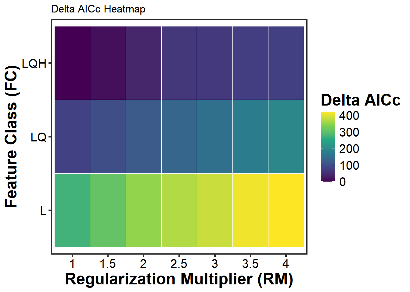
使用选出的最优 maxnet 模型,完成以下工作:
Boyce 曲线定量评估模型预测能力;得到最优模型和环境栅格后,使用terra::predict()即可对整个研究区进行空间预测。type = "cloglog"表示输出为互补双对数(complementary log-log)变换后的值,范围为 0–1,可解释为物种出现的相对概率。 * cloglog 与 logistic 的区别:MaxEnt 默认输出两种格式——logistic 和 cloglog。cloglog 是 Phillips et al.(2017)推荐的形式,它能更好地处理极低适生度区域的估计,且在生态学意义上更接近”出现概率”的直觉。
# 载入最佳模型
eval_model <- readr::read_rds(here("outputs", sp_target, "maxent_eval.rds"))
res <- eval_model@results
best_model <- eval_model@models[[which.min(eval_model@results$AICc)]] # 获取最优模型对象
best_model_id <- which.min(eval_model@results$AICc) # 获取最优模型的索引

pred_current <- terra::predict(
  bioclim,
  best_model, # 使用最优模型进行预测
  type = "cloglog", # 输出适生度指数(0-1)
  na.rm = TRUE # 删除NA值
)
|---------|---------|---------|---------|
=========================================
# 绘制最优模型的预测图表
plot(pred_current, main = "Predicted Suitability (Current Climate)") # 可视化当前气候下的适生度预测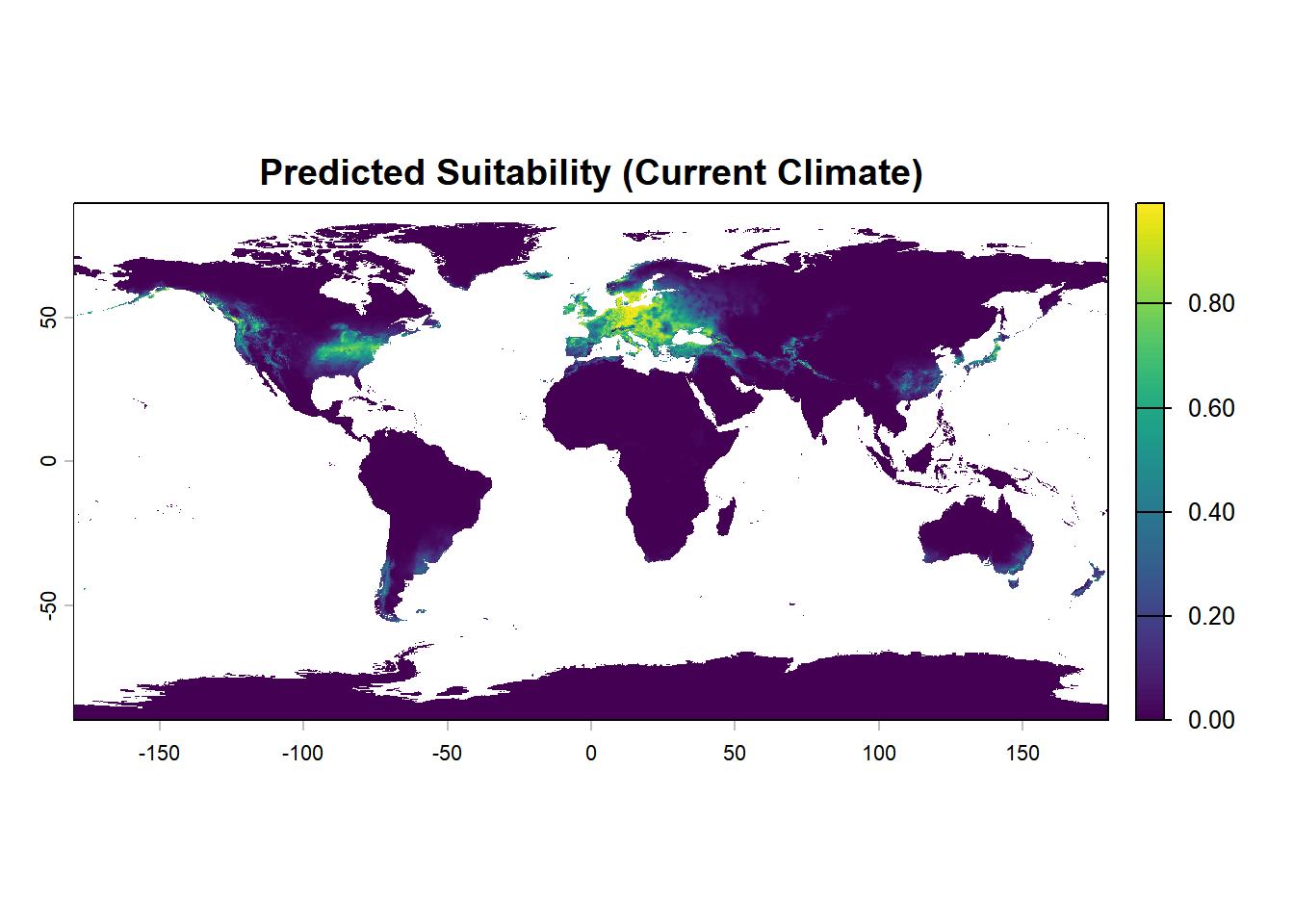
# 保存预测结果
terra::writeRaster(
  pred_current,
  filename = here(
    "outputs",
    sp_target,
    paste0("current_suitability_best_model_", best_model_id, ".tif")
  ),
  overwrite = TRUE
)首先从当前预测栅格中提取已知分布点位置的适生度值:
使用ecospat.boyce()函数计算Boyce指数:它通过将适生度值分成若干区间,计算每个区间内存在点的比例与该区间在整个预测栅格中的比例之比(Predicted/Expected ratio),并最终计算这些比值与适生度区间中点的 Spearman 秩相关系数。
boyce <- ecospat::ecospat.boyce(
  fit = fit_val, # 整个研究区的预测适生度值
  obs = pres_val, # 物种分布点处的预测适生度值
  nclass = 0, # 自动选择最优区间数
  window.w = "default", # 使用默认的滑动窗口宽度,用于平滑比值曲线
  res = 100, # 分辨率参数,控制计算精度
  PEplot = FALSE # 绘制Predicted/Expected比值曲线
)boyce_df <- data.frame(
HS = boyce$HS, # 适生度区间中点
Fratio = boyce$F.ratio # 预测/期望比值
)
boyce_plot <- ggplot(boyce_df, aes(x = HS, y = Fratio)) +
geom_line(color = "#2C7BB6", linewidth = 1.1) +
geom_point(size = 2, color = "#2C7BB7") +
geom_hline(yintercept = 1, linetype = "dashed", color = "red") +
labs(
title = "",
x = "Predicted Suitability (HS)",
y = "Predicted/Expected Ratio"
) +
annotate(
"text",
x = 0.25,
y = max(boyce_df$Fratio, na.rm = TRUE) * 0.9,
label = paste0("Boyce =", round(boyce$cor, 3)),
hjust = 1,
vjust = 1,
size = 5
) +
theme_bw() +
theme(
plot.title = element_text(hjust = 0.5, size = 16, face = "bold"),
axis.title = element_text(size = 14),
axis.text = element_text(size = 12)
)
boyce_plot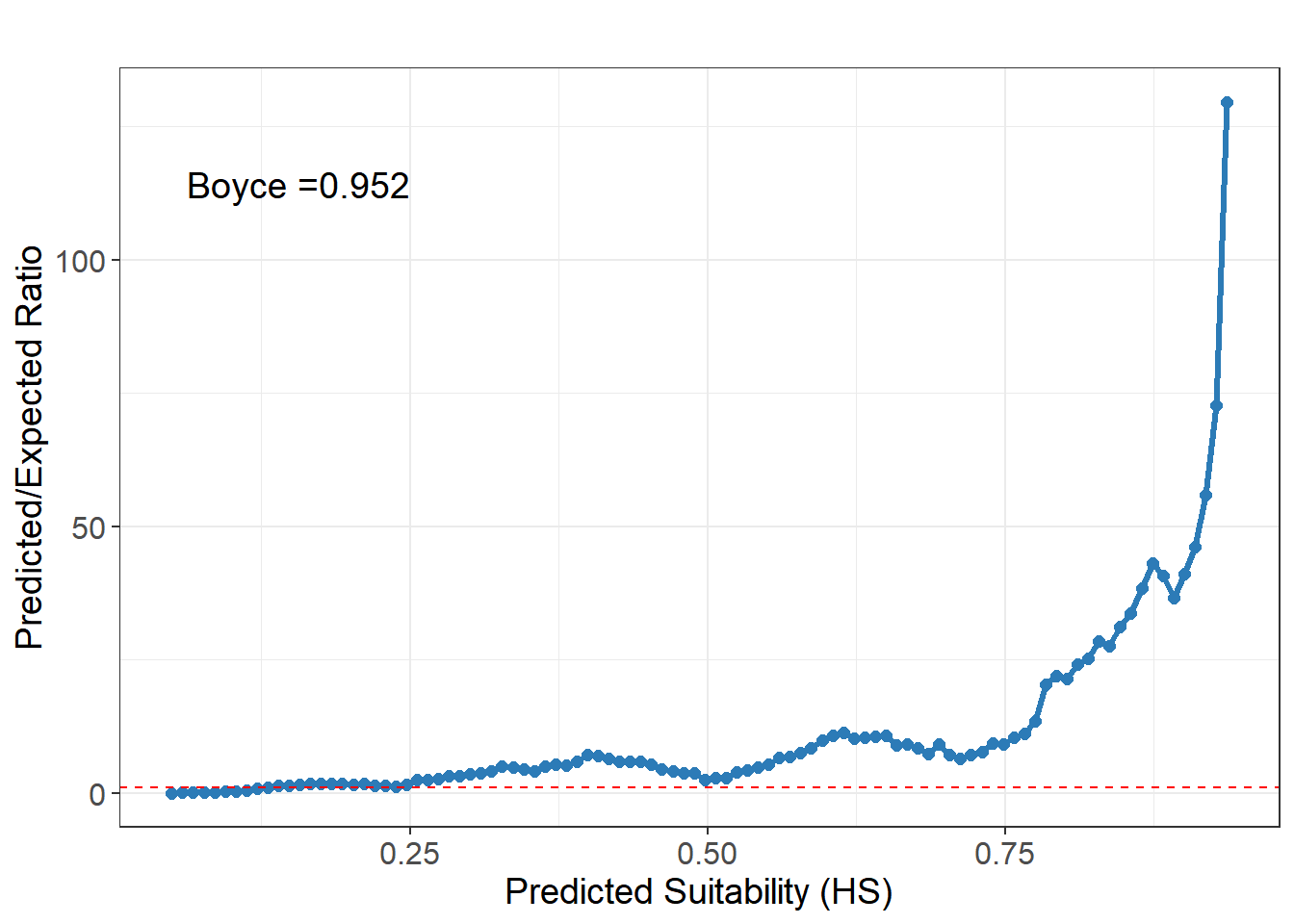
总体来讲:
跨时间投影的关键前提是变量名一致。未来气候栅格的波段名必须与模型训练时使用的变量名完全匹配,否则predict()会因找不到对应变量而报错。
# 读取未来气候数据
futrue_files <- list.files(
  here("datas", "SDM"),
  pattern = ".tif$",
  full.names = TRUE
)
env_future_all <- terra::rast(futrue_files)

# 统一变量名
future_bio_id <- gsub(".*_(\\d+)$", "\\1", names(env_future_all))
std_names <- paste0("bio_", future_bio_id, ".tif")
names(env_future_all) <- std_names
|---------|---------|---------|---------|
=========================================
toc()未来气候预测:: 64.73 sec elapsedplot(future_pred_ssp585, main = "Future Suitability")
# 保存未来气候下的适生度预测结果
terra::writeRaster(
  future_pred_ssp585,
  filename = here(
    "outputs",
    sp_target,
    paste0("future_ssp585_suitability_best_model_", "3", ".tif")
  ),
  overwrite = TRUE
)