遇到的问题和解法

1 使用ggtrendline包在图形中添加趋势线和置信区间

ggtrendline::ggtrendline()函数可以:

• 直接在图形中添加置信区间,趋势线和拟合公式(包括p值和r2).
• 可以和ggplot2中的geom_**()系列函数连用.

ggtrendline::ggtrendline()函数内置的模型公式如下:

$$\begin{array}{}\text{(1)}& line2P& :y=a\times x+b\text{(2)}& line3P& :y=a\times x^2+b\times x+c\text{(3)}& log2P& :y=a\times ln(x)+b\text{(4)}& exp2P& :y=a\times e^{b\times x}\text{(5)}& exp2P& :y=a\times e^{b\times x}\text{(6)}& exp3P& :y=a\times e^{b\times x}+c\text{(7)}& power2P& :y=a\times x^b\text{(8)}& power3P& :y=a\times x^b+c\end{array}$$

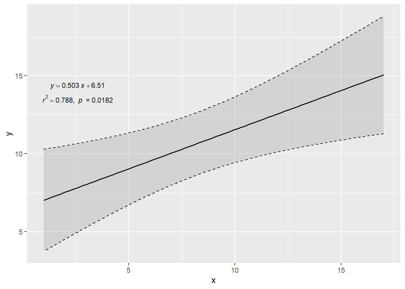
library(ggplot2)
library(ggtrendline)

# 例1
x <- c(1, 3, 6, 9, 13, 17)
y <- c(5, 8, 11, 13, 13.2, 13.5)
ggtrendline(x, y, model = "line2P")

Call:
lm(formula = y ~ x)

Residuals:
      1       2       3       4       5       6 
-2.0152 -0.0203  1.4721  1.9646  0.1545 -1.5556 

Coefficients:
            Estimate Std. Error t value Pr(>|t|)   
(Intercept)    6.513      1.286    5.07   0.0072 **
x              0.503      0.130    3.86   0.0182 * 
---
Signif. codes:  0 '***' 0.001 '**' 0.01 '*' 0.05 '.' 0.1 ' ' 1

Residual standard error: 1.77 on 4 degrees of freedom
Multiple R-squared:  0.788, Adjusted R-squared:  0.735 
F-statistic: 14.9 on 1 and 4 DF,  p-value: 0.0182


N: 6 , AIC: 27.4 , AICc: 39.4 , BIC:  26.8 
Residual Sum of Squares:  12.5 

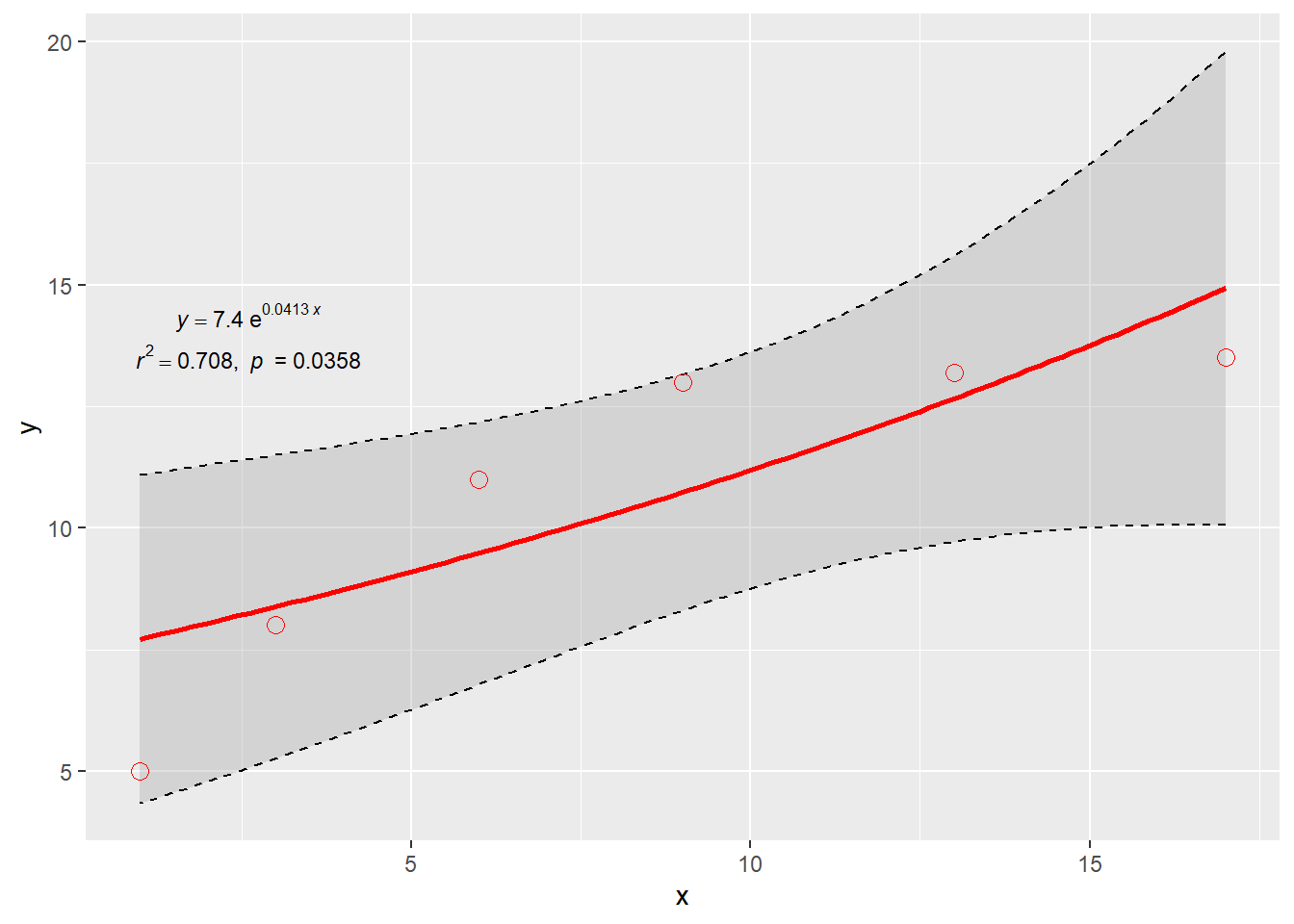
# 例2-设置回归线格式+与geom_**()函数连用
ggtrendline(x, y,
  model = "exp2P", linecolor = "red",
  linetype = 1, linewidth = 1
) +
  geom_point(aes(x, y), color = "red", shape = 1, size = 3)

Nonlinear regression model

Formula: y = a*exp(b*x) 

Parameters:
  Estimate Std. Error t value Pr(>|t|)   
a   7.4047     1.2602    5.88   0.0042 **
b   0.0413     0.0141    2.93   0.0429 * 
---
Signif. codes:  0 '***' 0.001 '**' 0.01 '*' 0.05 '.' 0.1 ' ' 1

Residual standard error: 2.08 on 4 degrees of freedom 

Number of iterations to convergence: 6
Achieved convergence tolerance: 1.76e-06 

Multiple R-squared: 0.708 , Adjusted R-squared:  0.635
F-statistic: 9.69 on 1 and 4 DF,  p-value: 0.0358 

N: 6 , AIC: 29.4 , AICc: 41.4 , BIC:  28.8 
Residual Sum of Squares:  17.3 

# 例3-设定置信区间
ggtrendline(x, y,
  model = "exp3P",
  CI.level = 0.99, CI.fill = "red", CI.alpha = 0.3, CI.color = NA,
  CI.lty = 2, CI.lwd = 1.5
) +
  geom_point(aes(x, y))

Nonlinear regression model

Formula: y = a*exp(b*x) + c 

Parameters:
  Estimate Std. Error t value Pr(>|t|)    
a -11.3682     0.5618  -20.24  0.00026 ***
b  -0.2360     0.0317   -7.45  0.00500 ** 
c  13.8551     0.3566   38.85  3.8e-05 ***
---
Signif. codes:  0 '***' 0.001 '**' 0.01 '*' 0.05 '.' 0.1 ' ' 1

Residual standard error: 0.357 on 3 degrees of freedom 

Number of iterations to convergence: 0
Achieved convergence tolerance: 2.59e-06 

Multiple R-squared: 0.994 , Adjusted R-squared:  0.989
F-statistic: 231 on 2 and 3 DF,  p-value: 0.000518 

N: 6 , AIC: 8.5 , AICc: 48.5 , BIC:  7.66 
Residual Sum of Squares:  0.382 

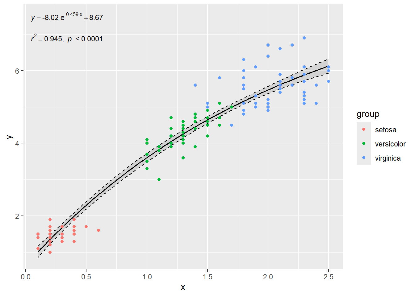
# 例4-分组拟合
x <- iris$Petal.Width
y <- iris$Petal.Length
group <- iris$Species

ggtrendline(x, y, model = "exp3P"
) +
  geom_point(aes(x, y, color = group))

Nonlinear regression model

Formula: y = a*exp(b*x) + c 

Parameters:
  Estimate Std. Error t value Pr(>|t|)    
a   -8.020      0.746  -10.75  < 2e-16 ***
b   -0.459      0.076   -6.04  1.2e-08 ***
c    8.674      0.803   10.80  < 2e-16 ***
---
Signif. codes:  0 '***' 0.001 '**' 0.01 '*' 0.05 '.' 0.1 ' ' 1

Residual standard error: 0.417 on 147 degrees of freedom 

Number of iterations to convergence: 4
Achieved convergence tolerance: 2.87e-06 

Multiple R-squared: 0.945 , Adjusted R-squared:  0.944
F-statistic: 1263 on 2 and 147 DF,  p-value: 2.63e-93 

N: 150 , AIC: 168 , AICc: 168 , BIC:  180 
Residual Sum of Squares:  25.5 

2 在图形中添加公式或其他数学注释

更多表达式语法:?plotmath

2.1 expression()函数

2.2 bquote()函数

library(tidyverse)
library(tibble)

# 模拟总体的正态分布：N(100, 15^2)
set.seed(42)
x <- rnorm(100000, mean = 100, sd = 15) # 100000个样本，均值为100，标准差为15
data <- as.data.frame(x)

# 抽样函数-抽取指定大小的样本，并计算其平均值及标准差
rnorm_stats <- function(df, n) {
  the_sample <- sample(x, n)
  tibble(
    sample_size = n,
    sample_mean = mean(the_sample),
    sample_sd = sd(the_sample)
  )
}

# 抽取2000个大小为10的样本，并计算其平均值及标准差 
df_sample_10 <-
  map_dfr(1:2000, \(x) rnorm_stats(x, 10))

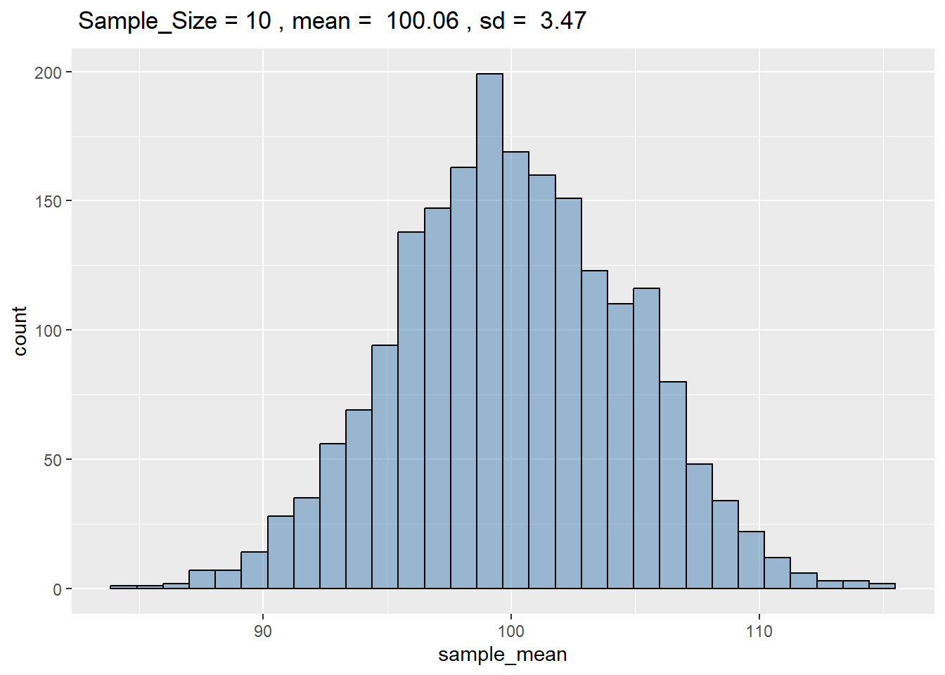
# 绘图-在标题中增加相关公式及数字。 
ggplot(df_sample_10, aes(x = sample_mean)) +
  geom_histogram(bins = 30, fill = "steelblue", color = "black", alpha = 0.5) +
  labs(
    title = bquote(
      ~"Sample_Size =" ~ 10
      ~ ", mean = " ~ .(round(mean(df_sample_10$sample_mean), 2))
      ~ ", sd = " ~ .(round(sd(df_sample_10$sample_sd), 2))
    )
  )

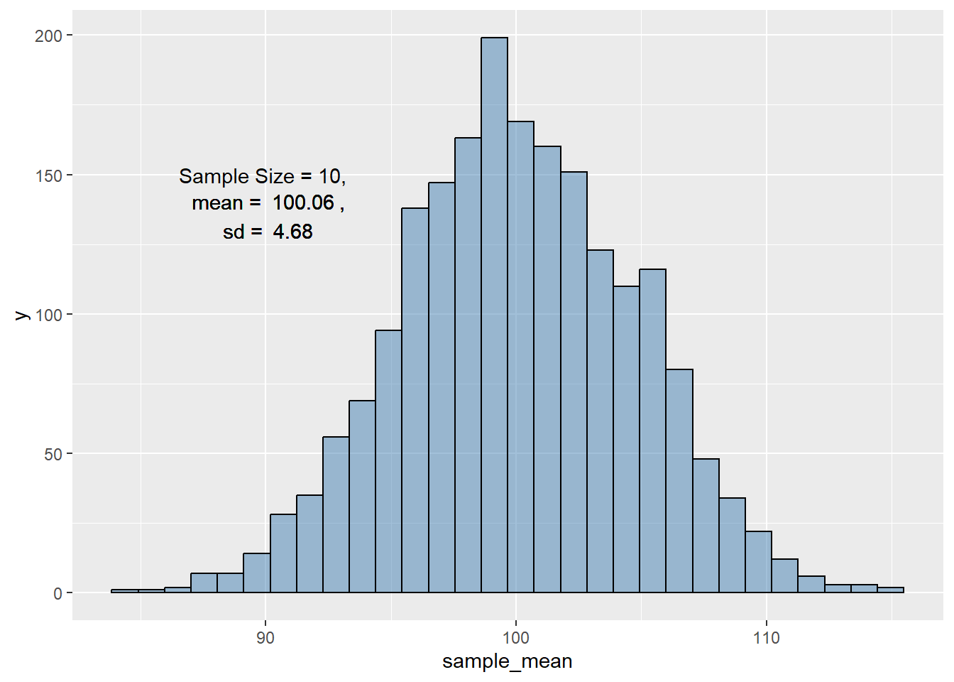
# 绘图-在图形中添加相关公式及数字
e <- "Sample Size = 10"
ggplot(df_sample_10, aes(x = sample_mean)) +
  geom_histogram(bins = 30, fill = "steelblue", color = "black", alpha = 0.5) +
  annotate("text", 90, 150, label = bquote("Sample Size = 10, ")) +
  annotate("text", 90, 140,
    label = bquote(~"mean = "~ .(round(mean(df_sample_10$sample_mean), 2))
    ~",")
  ) +
  annotate("text", 90, 130,
    label = bquote(~"sd = "~  .(round(sd(df_sample_10$sample_mean), 2)))
  )

3 列联表