1 第一步:记住几个重要参数的清单
-
字体:
Arial或Helvetica,正文11pt,标题12pt。 -
主题:黑白主题,
theme_classic(),无网格背景。 -
分辨率:
300 DPI以上。 -
格式:
TIFF(首选)或EPS。 -
尺寸:单栏图约
3.5英寸,双栏图约7.5英寸。 - 配色:适合黑白印刷(灰度配色)或色盲友好配色。
- 图例:优先放图内,不在图外单独占空间。
把这个清单保存下来,每次画图的时候粘进提示词,DeepSeek V4给你的代码就直接是投稿级别的。
2 第二步:通用的图标导出函数
每次画完图都要导出,把这个函数放在脚本最前面,之后直接调用:
# 投稿级的图表导出函数
save_figure <- function(
  plot,
  filename,
  width = 7,
  height = 5,
  dpi = 300,
  device = "jpg"
) {
  ggsave(
    filename = here("outputs", "figures", paste0(filename, ".", device)),
    plot = plot,
    width = width,
    height = height,
    units = "in",
    dpi = dpi,
    device = device
  )
  message("✅ 图表已保存:", filename, ".", device)
}
3 第三步:投稿的通用主题theme
把这个主题对象放在脚本里,每张图都加上+ theme_publication():
theme_publication <- function(base_size = 11, base_family = "Arial") {
  theme_classic(base_size = base_size, base_family = base_family) +
    theme_sub_legend(
      title = element_text(size = base_size, face = "bold"),
      text = element_text(size = base_size - 1),
      background = element_rect(fill = "white", color = "grey80", linewidth = 0.3),
      key.size = unit(0.4, "cm")
    ) +
    theme_sub_plot(
      title = element_text(size = base_size + 1, face = "bold", hjust = 0.5),
      margin = margin(10, 15, 10, 10),
      background = element_rect(fill = "white", color = NA),
    ) +
    theme_sub_axis(
      title = element_text(size = base_size, face = "bold"),
      text = element_text(size = base_size - 1, color = "black")
    ) +
    theme_sub_panel(background = element_rect(fill = "white", color = NA)) +
    theme(
      # 文字
      text = element_text(family = base_family, size = base_size),
    )
}
4 类型一:散点图
最常用场景:探索两个连续变量之间的关系,展示相关性,添加回归线。
# A tibble: 6 × 12
  car            mpg cyl    disp    hp  drat    wt  qsec    vs    am  gear  carb
  <chr>        <dbl> <fct> <dbl> <dbl> <dbl> <dbl> <dbl> <dbl> <dbl> <dbl> <dbl>
1 Mazda RX4     21   6 缸    160   110  3.9   2.62  16.5     0     1     4     4
2 Mazda RX4 W…  21   6 缸    160   110  3.9   2.88  17.0     0     1     4     4
3 Datsun 710    22.8 4 缸    108    93  3.85  2.32  18.6     1     1     4     1
4 Hornet 4 Dr…  21.4 6 缸    258   110  3.08  3.22  19.4     1     0     3     1
5 Hornet Spor…  18.7 8 缸    360   175  3.15  3.44  17.0     0     0     3     2
6 Valiant       18.1 6 缸    225   105  2.76  3.46  20.2     1     0     3     1
# 基础散点图
p_scatter_basic <- ggplot(mtcars_df, aes(x = wt, y = mpg)) +
geom_point(aes(color = cyl, shape = cyl), size = 2.5, alpha = 0.8) +
geom_smooth(
aes(group = 1),
method = "lm",
se = T,
color = "black",
linewidth = 0.8,
alpha = 0.15
)
p_scatter_basic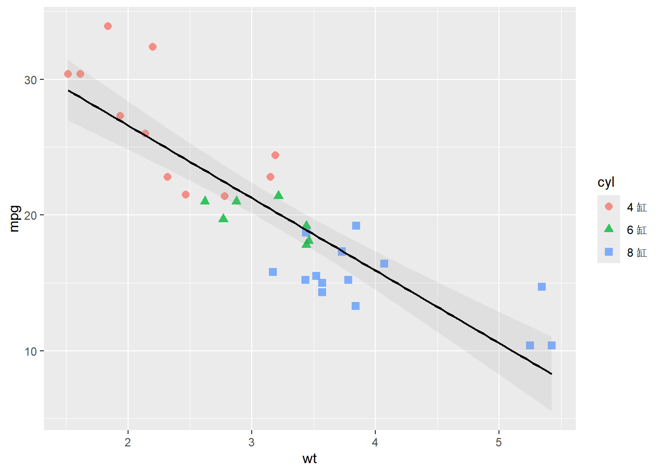
# 加入投稿级配色,应用投稿主题
p_scatter <- p_scatter_basic +
  ggsci::scale_color_lancet() + # ggsici提供的Lancet配色方案,适合科学图表
  theme_publication() +
  theme(
    legend.position = c(0.85, 0.85) # 将图例放在图内右上角
  ) +
  labs(
    x = "车重 (wt)",
    y = "每加仑英里数 (mpg)",
    color = "气缸数",
    shape = "气缸数",
    title = NULL
  )
p_scatter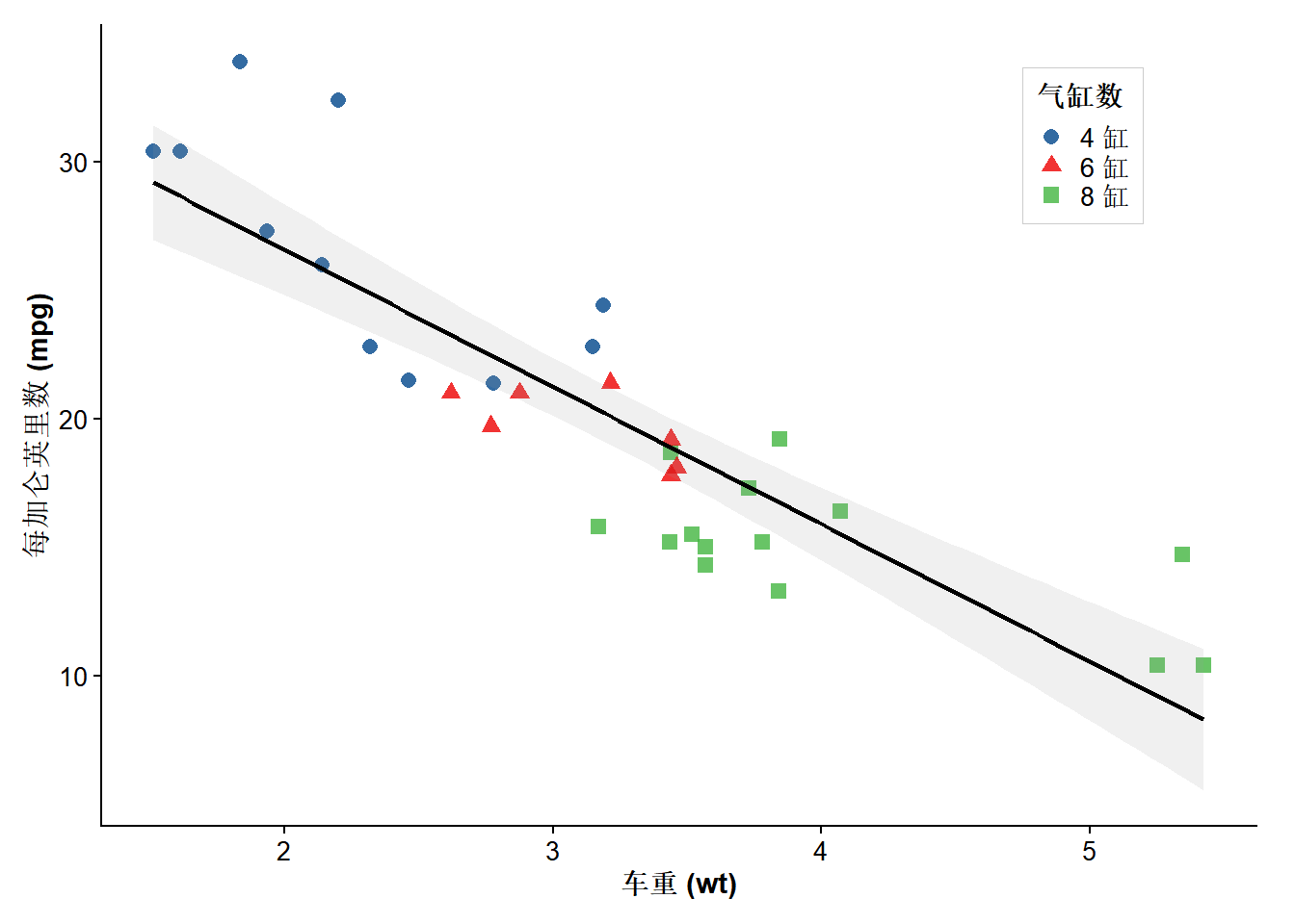
# 导出图表
save_figure(p_scatter, "fig1_scatter")
5 类型二:箱线图
最常用场景:比较多个组的连续变量分布,展示中位数、四分位数和异常值。
p_boxplot_basic <- ggplot(iris, aes(x = Species, y = Sepal.Length, fill = Species)) +
  geom_boxplot(
    alpha = 0.7,
    outlier.shape = 21, # 使用空心圆表示异常值
    outlier.size = 1.5,
    outlier.alpha = 0.6,
    width = 0.5
  ) +
  # 添加散点以显示数据分布,使用jitter避免重叠
  geom_jitter(width = 0.15, alpha = 0.4, size = 1)
p_boxplot_basic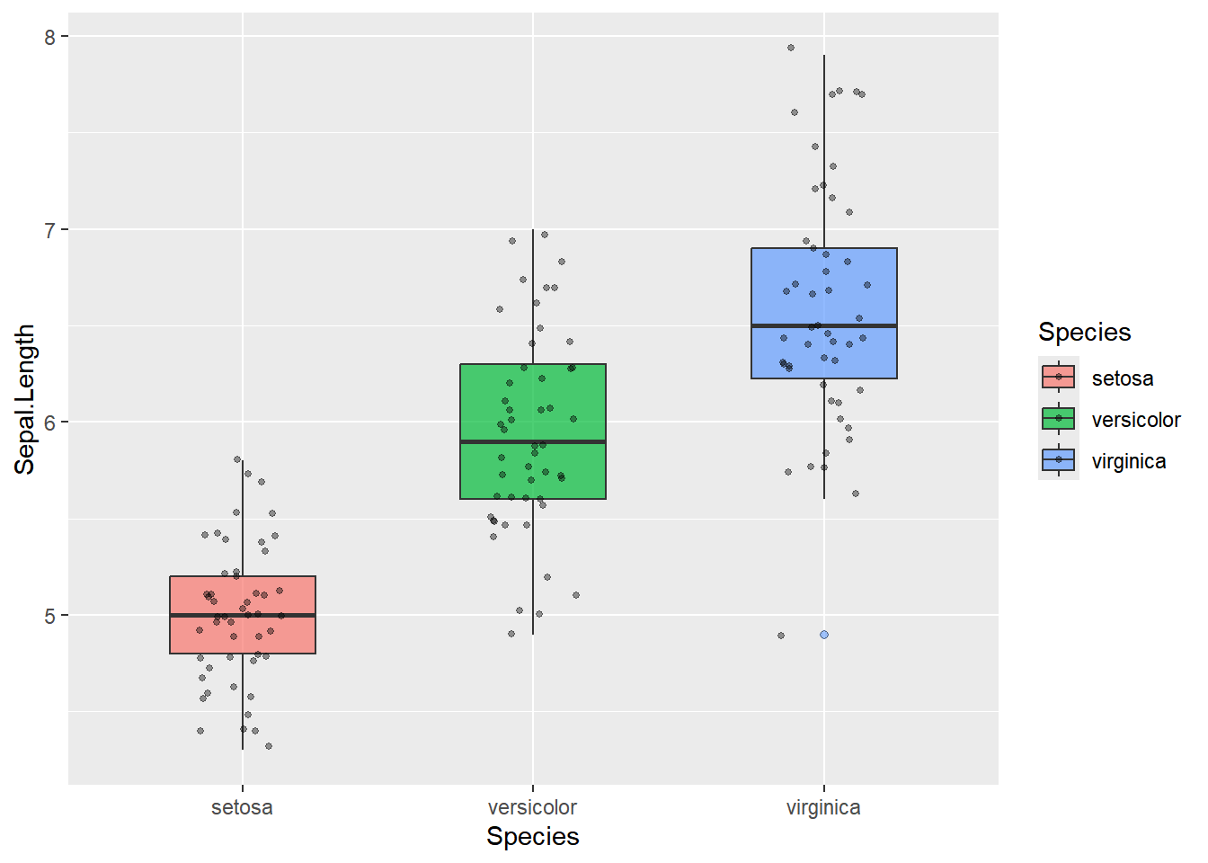
# 加入投稿级配色,应用投稿主题
p_boxplot <- p_boxplot_basic +
  ggsci::scale_fill_lancet() + # 使用Lancet配色方案
  theme_publication() +
  theme(
    legend.position = "none" # 分组已经在x轴和颜色显示,不显示图例
  ) +
  labs(x = "物种", y = "花萼长度 (cm)", title = NULL)
p_boxplot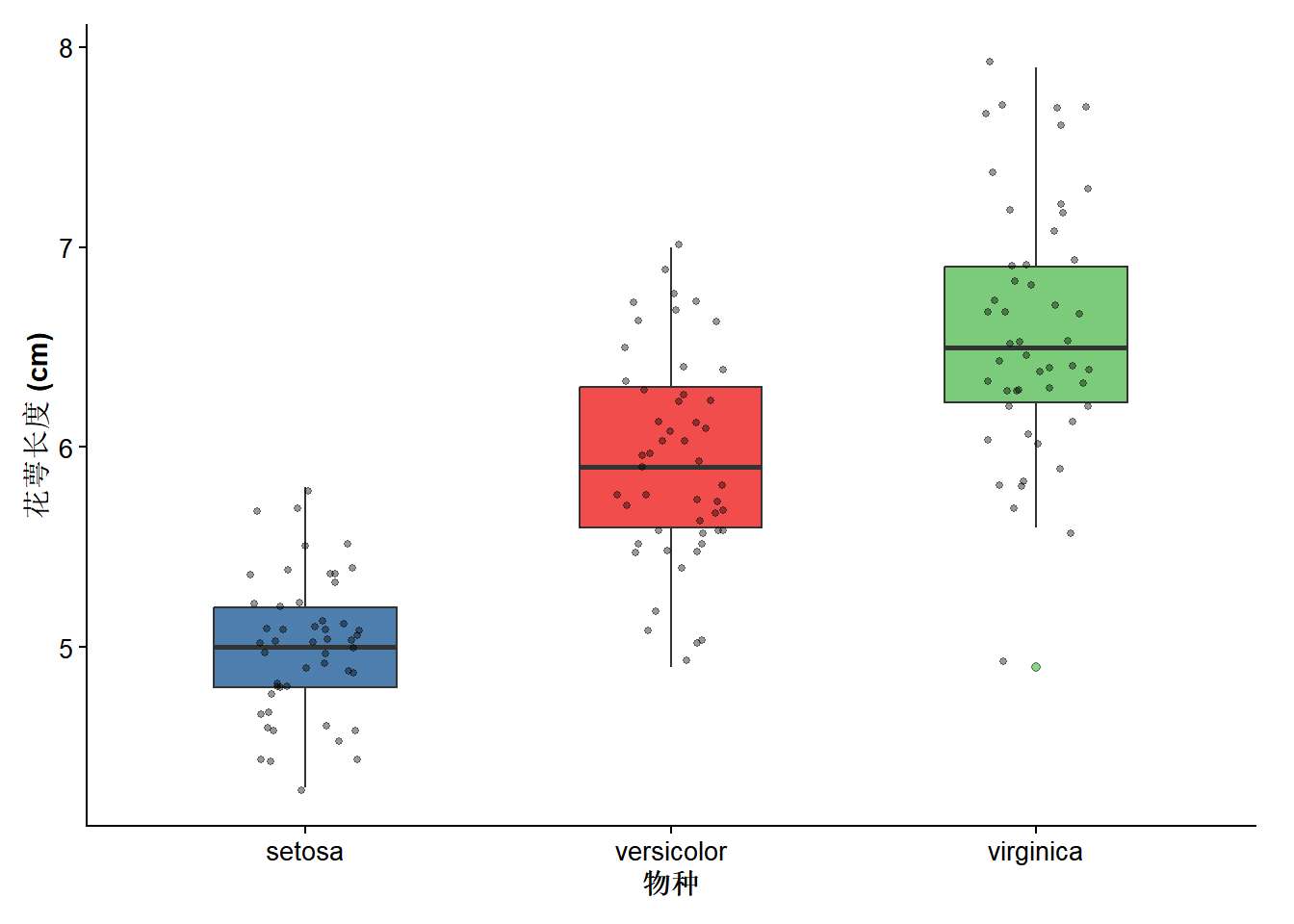
# 在箱线图中加入统计显著性标记
p_boxplot_stat <- p_boxplot +
  ggpubr::stat_compare_means(
    method = "wilcox.test",
    comparisons = list(
      c("setosa", "versicolor"),
      c("setosa", "virginica"),
      c("versicolor", "virginica")
    ),
    label = "p.signif", # p.singificant显示星号,p.format显示具体p值
    label.y = c(7, 7.5, 8), # 调整显著性标记的位置
    step.increase = 0.1 # 每个比较之间增加10%的高度,避免重叠
  )
p_boxplot_stat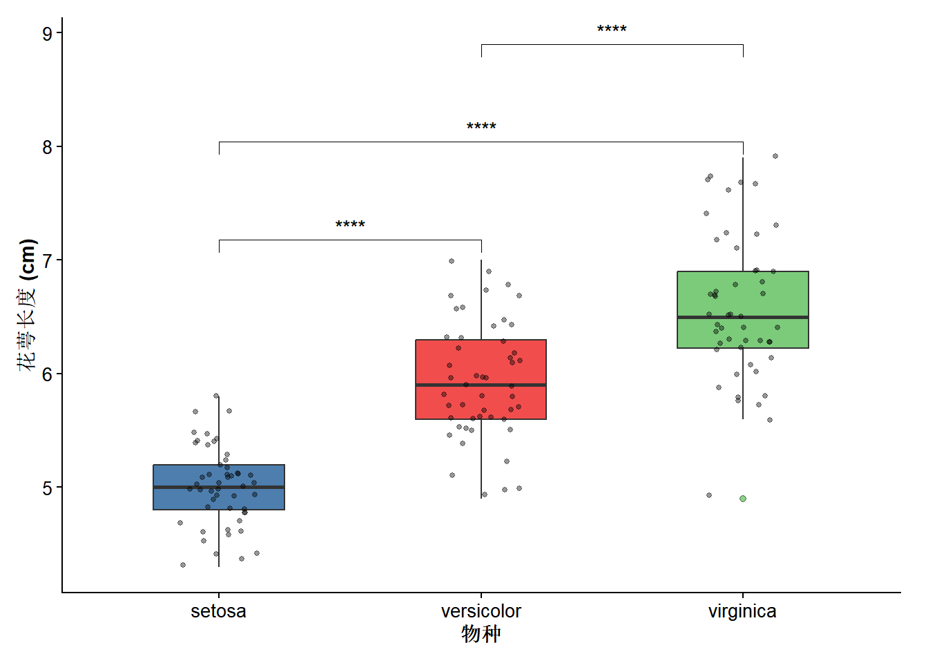
# 导出图表
save_figure(p_boxplot_stat, "fig2_boxplot")
6 类型三:柱状图
最常用场景:比较不同组的均值或总和,展示分类变量的分布。
p_bar_df <- iris |>
  group_by(Species) |>
  summarise(mean_sl = mean(Sepal.Length), se_sl = sd(Sepal.Length) / sqrt(n()))

# 基础柱状图--显示均值和误差线
p_bar_basic <- ggplot(p_bar_df, aes(x = Species, y = mean_sl, fill = Species)) +
  geom_col(width = 0.6, alpha = 0.5) +
  # 误差棒
  geom_errorbar(
    aes(ymin = mean_sl - se_sl, ymax = mean_sl + se_sl),
    width = 0.2,
    # color = "black",
    linewidth = 0.7
  )
p_bar_basic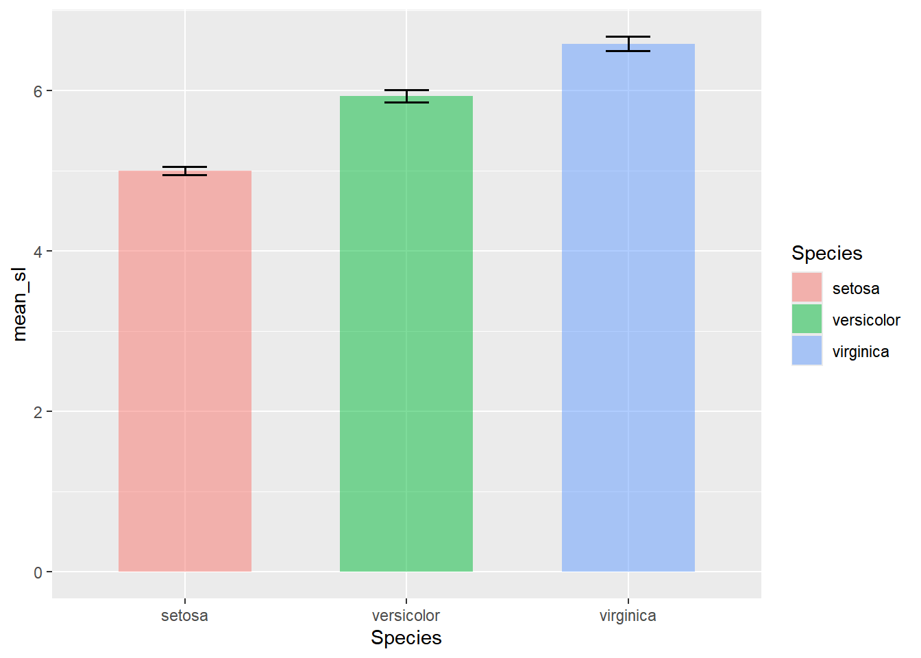
# 加入投稿级配色,应用投稿主题
p_bar <- p_bar_basic +
  ggsci::scale_fill_lancet() + # 使用Lancet配色方案
  theme_publication() +
  theme(
    legend.position = "none" # 分组已经在x轴和颜色显示,不显示图例
  ) +
  scale_y_continuous(expand = expansion(mult = c(0, 0.1))) + # 调整y轴起点为0,增加10%空间
  labs(x = "物种", y = "花萼长度均值 (cm ± SE)", title = NULL)
p_bar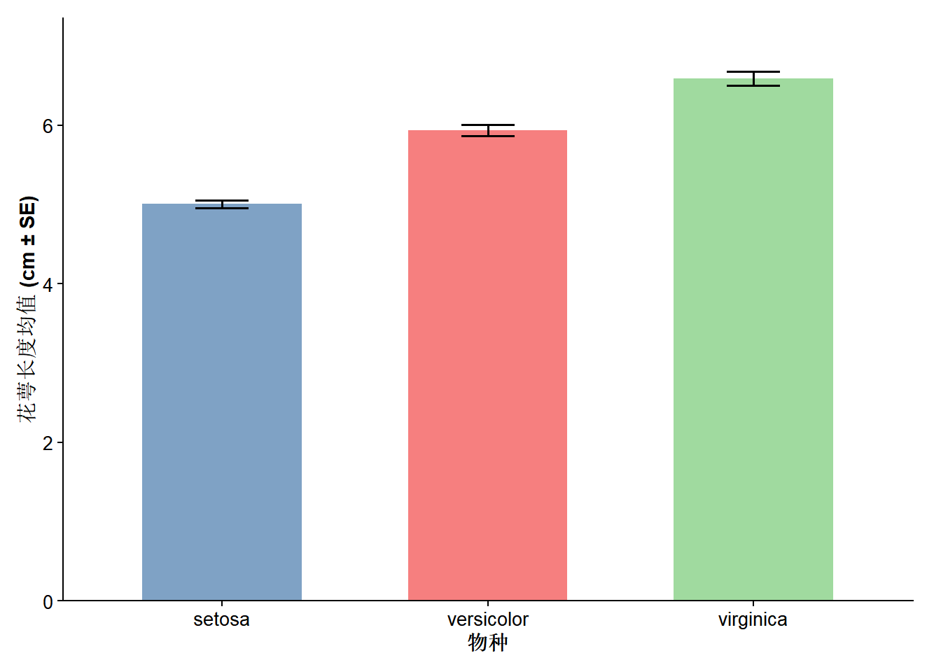
# 导出图表
save_figure(p_bar, "fig3_bar")
7 类型四:折线图
最常用场景:展示随时间或其他连续变量变化的趋势,多组对比。
# 构造示例数据

set.seed(42)
followup_data <- expand.grid(
  time = c(0, 3, 6, 9, 12),
  group = c("治疗组", "对照组")
) |>
  mutate(
    # fmt: skip
    mean_score = c(
      50, 45, 38, 30, 25, # 治疗组: time 0,3,6,9,12
      50, 49, 48, 47, 46), # 对照组: time 0,3,6,9,12
    se = c(3, 3, 2.5, 2, 2, 3, 3, 3, 3, 3)
  )

# 基础折线图-显示置信区间
p_line_basic <- ggplot(
  followup_data,
  aes(x = time, y = mean_score, color = group, shape = group)
) +
  geom_line(linewidth = 0.9) +
  geom_point(size = 3) +
  geom_ribbon(
    # 添加置信区间
    aes(ymin = mean_score - se, ymax = mean_score + se, fill = group),
    alpha = 0.15,
    color = NA
  )
p_line_basic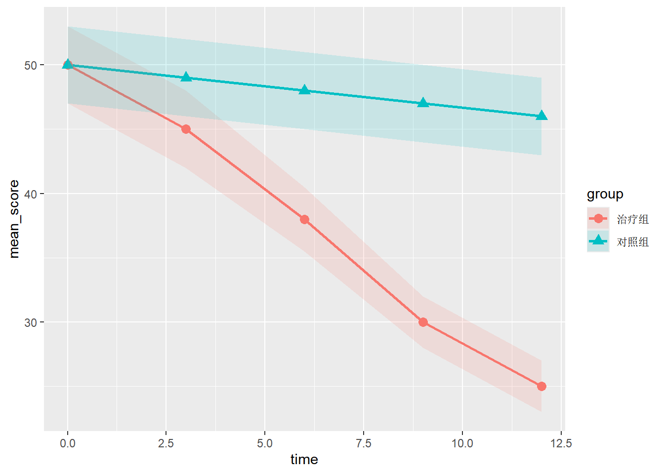
# 加入投稿级配色,应用投稿主题
p_line <- p_line_basic +
  ggsci::scale_color_lancet() + # 使用Lancet配色方案
  ggsci::scale_fill_lancet() + # 填充颜色与线条颜色一致
  theme_publication() +
  theme(
    legend.position = c(0.85, 0.5) # 将图例放在图内右上角
  ) +
  labs(
    x = "随访时间 (月)",
    y = "平均评分 (分值 ± SE)",
    color = "治疗方案",
    shape = "治疗方案",
    fill = "治疗方案",
    title = NULL
  )
p_line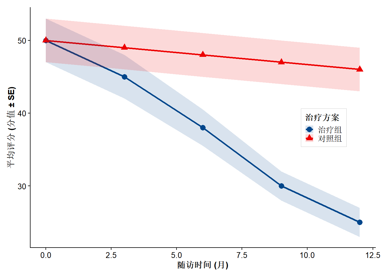
# 导出图表
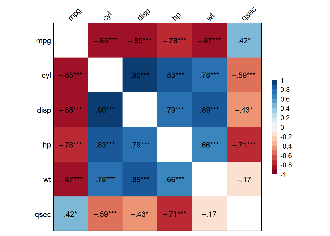
save_figure(p_line, "fig4_line")8 类型四:热图
最常用场景:相关矩阵可视化,基因表达热图,样本聚类分析。
Pearson's r and 95% confidence intervals:
────────────────────────────────────────────
               r       [95% CI]     p      N
────────────────────────────────────────────
mpg-cyl    -0.85 [-0.93, -0.72] <.001 *** 32
mpg-disp   -0.85 [-0.92, -0.71] <.001 *** 32
mpg-hp     -0.78 [-0.89, -0.59] <.001 *** 32
mpg-wt     -0.87 [-0.93, -0.74] <.001 *** 32
mpg-qsec    0.42 [ 0.08,  0.67]  .017 *   32
cyl-disp    0.90 [ 0.81,  0.95] <.001 *** 32
cyl-hp      0.83 [ 0.68,  0.92] <.001 *** 32
cyl-wt      0.78 [ 0.60,  0.89] <.001 *** 32
cyl-qsec   -0.59 [-0.78, -0.31] <.001 *** 32
disp-hp     0.79 [ 0.61,  0.89] <.001 *** 32
disp-wt     0.89 [ 0.78,  0.94] <.001 *** 32
disp-qsec  -0.43 [-0.68, -0.10]  .013 *   32
hp-wt       0.66 [ 0.40,  0.82] <.001 *** 32
hp-qsec    -0.71 [-0.85, -0.48] <.001 *** 32
wt-qsec    -0.17 [-0.49,  0.19]  .339     32
────────────────────────────────────────────
# 导出图表
save_figure(p_heatmap, "fig5_heatmap")
9 类型五:火山图
最常用场景:差异分析结果可视化,展示基因表达变化的显著性和效应大小。它能把“变化幅度”和“显著性”放在同一张图里,快速筛出值得关注的因子、指标或特征。
# 构造示例数据
set.seed(42)
n_genes <- 2000
volcano_data <- data.frame(
  gene = paste0("Gene", 1:n_genes),
  log2FC = rnorm(n_genes, 0, 1.5),
  neg_log10_p = rchisq(n_genes, df = 2)
) |>
  mutate(
    # 定义显著性分类
    significance = case_when(
      log2FC > 1 & neg_log10_p > -log10(0.05) ~ "上调",
      log2FC < -1 & neg_log10_p > -log10(0.05) ~ "下调",
      TRUE ~ "不显著"
    ),
    # 标记最显著的基因
    label = ifelse(
      neg_log10_p > quantile(neg_log10_p, 0.98) & abs(log2FC) > 1,
      gene,
      NA
    )
  )

# 统计各类数量
sig_counts <- table(volcano_data$significance)

# 基础火山图
p_volcano_basic <- ggplot(
  volcano_data,
  aes(x = log2FC, y = neg_log10_p, color = significance)
) +
  # 不显著点-先画,所以在底层
  geom_point(
    data = filter(volcano_data, significance == "不显著"),
    size = 0.8,
    alpha = 0.4
  ) +
  # 显著点-后画,所以在上层
  geom_point(
    data = filter(volcano_data, significance != "不显著"),
    size = 1.2,
    alpha = 0.8
  ) +
  # 添加显著性阈值线
  geom_vline(
    xintercept = c(-1, 1),
    color = "grey50",
    linetype = "dashed",
    linewidth = 0.5
  ) +
  geom_hline(
    yintercept = -log10(0.05),
    color = "grey50",
    linetype = "dashed",
    linewidth = 0.5
  )
p_volcano_basic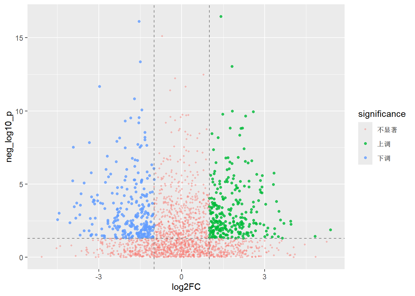
# 加入投稿级配色,应用投稿主题
p_volcano <- p_volcano_basic +
  scale_color_manual(
    values = c(
      "上调" = "#E41A1C", # 红色
      "下调" = "#377EB8", # 蓝色
      "不显著" = "#AAAAAA" # 灰色
    ),
    labels = c(
      "上调" = paste0("上调 (n=", sig_counts["上调"], ")"),
      "下调" = paste0("下调 (n=", sig_counts["下调"], ")"),
      "不显著" = paste0("不显著 (n=", sig_counts["不显著"], ")")
    )
  ) +
  # 标注显著的点名
  ggrepel::geom_text_repel(
    aes(label = label),
    size = 3,
    max.overlaps = 10,
    box.padding = 0.5,
    point.padding = 0.5,
    segment.color = "grey80",
    show.legend = FALSE
  ) +
  theme_publication() +
  labs(
    x = expression(log[2] * "Fold Change"),
    y = expression(-log[10] * ("P-value")),
    color = "显著性差异"
  )
p_volcano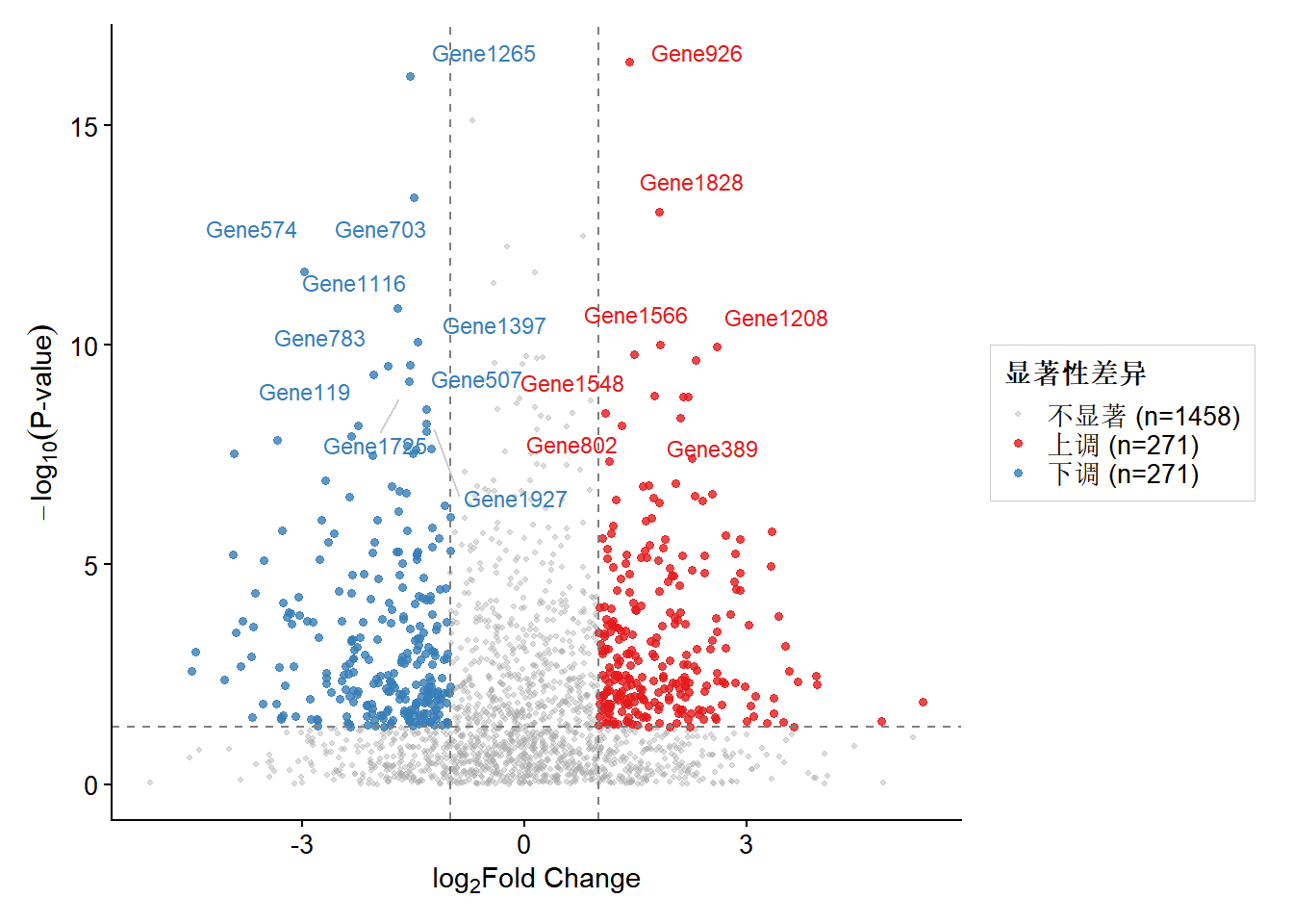
# 图形导出
save_figure(p_volcano, "fig6_volcano", dpi = 300)