ggplot2中有丰富的作图函数和技巧。我们挑出常用、重点的聊聊。
1 坐标系统
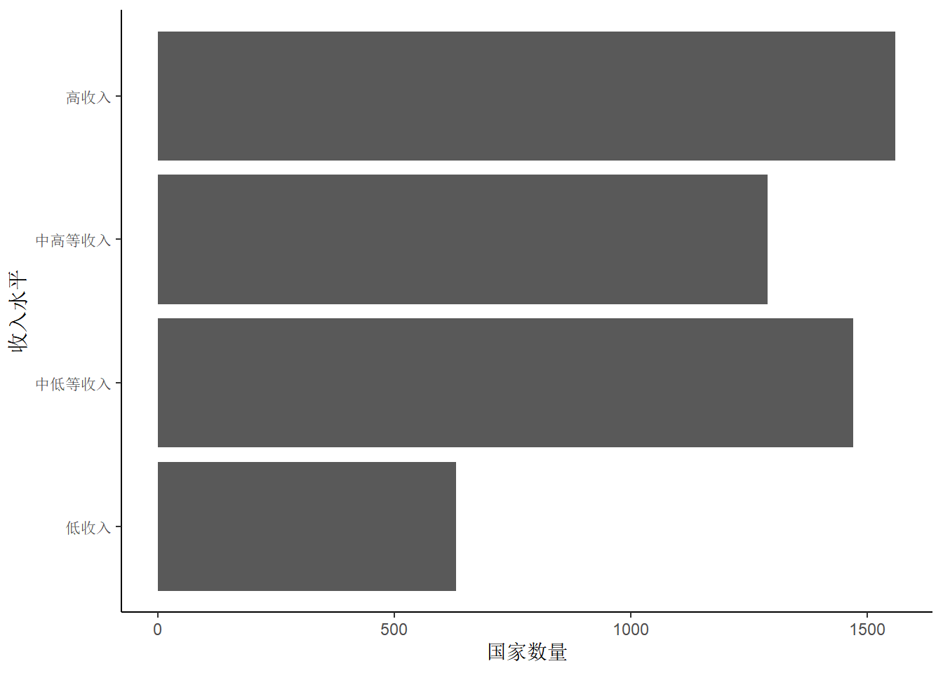
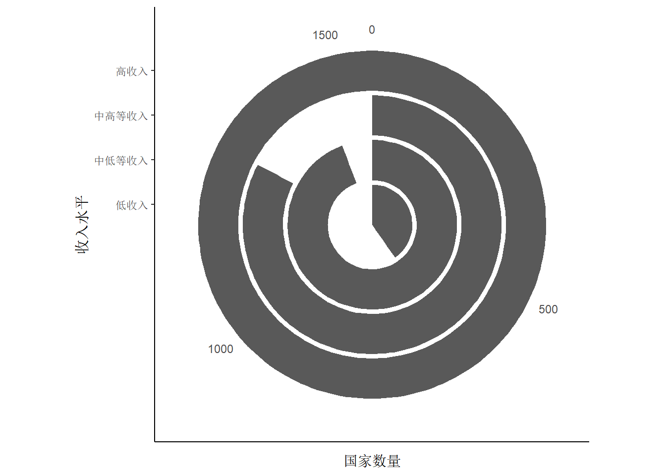
不同坐标系下的柱状图、条形图、饼图。
Note
值得注意的是,ggplot2中没有直接绘制饼图的函数(Hadley认为饼图并不能很好的展示数据),只能通过极坐标转换。
library(scales)
gapminder_2007 <- gapminder %>%
  filter(year == 2007)

ggplot(gapminder, aes(x = income_level)) +
  geom_bar(stat = "count") +
  theme_classic() +
  labs(x = "收入水平", y = "国家数量")

ggplot(gapminder, aes(x = income_level)) +
  geom_bar(stat = "count") +
  coord_flip() +  # 坐标轴翻转
  theme_classic() +
  labs(x = "收入水平", y = "国家数量")

ggplot(gapminder, aes(x = income_level)) +
  geom_bar(stat = "count") +
  coord_polar(theta = "x") +  # 极坐标转化:x轴转化,其中参数theta = "x"可省略
  theme_classic() +
  labs(x = "收入水平", y = "国家数量")

ggplot(gapminder, aes(x = income_level)) +
  geom_bar(stat = "count") +
  coord_polar(theta = "y") +  # 极坐标转化:y轴转化
  theme_classic() +
  labs(x = "收入水平", y = "国家数量")

以上图形中均可以加入分组情况,如希望按照地区分组,只需在参数aes()中加入fill = region即可。
2 插入公式
有时,我们需要在图片中插入公式使得图片的展示效果达到最佳。相比ggplot2中自带的插入公式的方法,我更习惯latex2exp输入的公式的方式。
例如,我们如何在ggplot2图形中插入如下公式(形状参数分别为a和b的贝塔分布的概率密度函数):
\[ f(x;a,b) = \frac{\Gamma(a+b)}{\Gamma(a)\Gamma(b)}x^{a-1}(1-x)^{b-1}, \quad a>0,b>0,0\leq x \leq 1 \]
library(latex2exp)

ggplot() +
  geom_function(
    fun = dbeta, args = list(shape1 = 3, shape2 = 0.9),
    colour = "#E41A1C", linewidth = 1.2,
  ) +
  geom_function(
    fun = dbeta, args = list(shape1 = 3, shape2 = 9),
    colour = "#377EB8", linewidth = 1.2
  ) +
  theme_classic() +
  labs(
    x = TeX(r'($x$)'), y = TeX(r'($f(x)$)'),
    title = TeX(r'($f(x) = \frac{\Gamma(a+b)}{\Gamma(a)\Gamma(b)}x^{a-1}(1-x)^{b-1}$)')
  )