library(tidyverse) # metapackage of all tidyverse packages
library(ggplot2)
library(dplyr)
library(reshape2) # Melt
library(plyr)

library(scales) # visualisation
library(corrplot) # visualisation
library(GGally) # visualisation
library(ggthemes) # visualisation
library(ggalt) # encircle
library(maps) # maps
library(treemap)
library(ggdendro) # Dendogram

# Interactivity
library(crosstalk)
library(plotly)

# Date
library(scales)
library(zoo)
library(lubridate)

# Function to plot width and height of plot
fig <- function(x, y) {
  options(repr.plot.width = x, repr.plot.height = y)
}
# load data
gapminder <- read_rds(file = "d:/Myblog/datas/gapminder-2020.rds")
titanic <- read_csv("d:/Myblog/datas/ggplot2cheetsheet/titanic/train.csv", show_col_types = FALSE)
insurance <- read_csv("d:/Myblog/datas/ggplot2cheetsheet/health-insurance-cross-sell-prediction/train.csv", show_col_types = FALSE)
university <- read_csv("d:/Myblog/datas/ggplot2cheetsheet/world-university-rankings/cwurData.csv", show_col_types = FALSE)
house <- read_csv("d:/Myblog/datas/ggplot2cheetsheet/house-prices-advanced-regression-techniques/train.csv", show_col_types = FALSE)
health <- read_csv("d:/Myblog/datas/ggplot2cheetsheet/av-healthcare-analytics-ii/healthcare/train_data.csv", show_col_types = FALSE)
netflix <- read_csv("d:/Myblog/datas/ggplot2cheetsheet/netflix-shows/netflix_titles.csv", show_col_types = FALSE)
playstore <- read_csv("d:/Myblog/datas/ggplot2cheetsheet/google-play-store-apps/googleplaystore.csv", show_col_types = FALSE)
covid <- read_csv("d:/Myblog/datas/ggplot2cheetsheet/novel-corona-virus-2019-dataset/covid_19_data.csv", show_col_types = FALSE)
campus <- read_csv("d:/Myblog/datas/ggplot2cheetsheet/Placement_Data_Full_Class.csv", show_col_types = FALSE)
police <- read_csv("d:/Myblog/datas/ggplot2cheetsheet/us-police-shootings/shootings.csv", show_col_types = FALSE)
axis <- read_csv("d:/Myblog/datas/ggplot2cheetsheet/nifty50-stock-market-data/AXISBANK.csv", show_col_types = FALSE)
hdfc <- read_csv("d:/Myblog/datas/ggplot2cheetsheet/nifty50-stock-market-data/HDFCBANK.csv", show_col_types = FALSE)
indus <- read_csv("d:/Myblog/datas/ggplot2cheetsheet/nifty50-stock-market-data/INDUSINDBK.csv", show_col_types = FALSE)
kotak <- read_csv("d:/Myblog/datas/ggplot2cheetsheet/nifty50-stock-market-data/KOTAKBANK.csv", show_col_types = FALSE)
icici <- read_csv("d:/Myblog/datas/ggplot2cheetsheet/nifty50-stock-market-data/ICICIBANK.csv", show_col_types = FALSE)
cipla <- read_csv("d:/Myblog/datas/ggplot2cheetsheet/nifty50-stock-market-data/CIPLA.csv", show_col_types = FALSE)
nifty <- read_csv("d:/Myblog/datas/ggplot2cheetsheet/nifty50-stock-market-data/NIFTY50_all.csv", show_col_types = FALSE)
space <- read_csv("d:/Myblog/datas/ggplot2cheetsheet/Space_Corrected.csv", show_col_types = FALSE)
windows <- read_csv("d:/Myblog/datas/ggplot2cheetsheet/windows-store/msft.csv", show_col_types = FALSE)
aqi <- read_csv("d:/Myblog/datas/ggplot2cheetsheet/india-air-quality-data/data.csv", show_col_types = FALSE)
stack <- read_csv("d:/Myblog/datas/ggplot2cheetsheet/60k-stack-overflow-questions-with-quality-rate/train.csv", show_col_types = FALSE)
delhi_house <- read_csv("d:/Myblog/datas/ggplot2cheetsheet/housing-prices-in-metropolitan-areas-of-india/Delhi.csv", show_col_types = FALSE)
climate <- read_csv("d:/Myblog/datas/ggplot2cheetsheet/climate-change-earth-surface-temperature-data/GlobalLandTemperaturesByCountry.csv", show_col_types = FALSE)
chennai_house <- read_csv("d:/Myblog/datas/ggplot2cheetsheet/housing-prices-in-metropolitan-areas-of-india/Chennai.csv", show_col_types = FALSE)
bangalore_house <- read_csv("d:/Myblog/datas/ggplot2cheetsheet/housing-prices-in-metropolitan-areas-of-india/Bangalore.csv", show_col_types = FALSE)
itc <- read_csv("d:/Myblog/datas/ggplot2cheetsheet/nifty50-stock-market-data/ITC.csv", show_col_types = FALSE)
covid_usa <- read_csv("d:/Myblog/datas/ggplot2cheetsheet/covid19-in-usa/us_counties_covid19_daily.csv", show_col_types = FALSE)ggplot2中有丰富的作图函数和技巧。我们挑出常用、重点的聊聊。
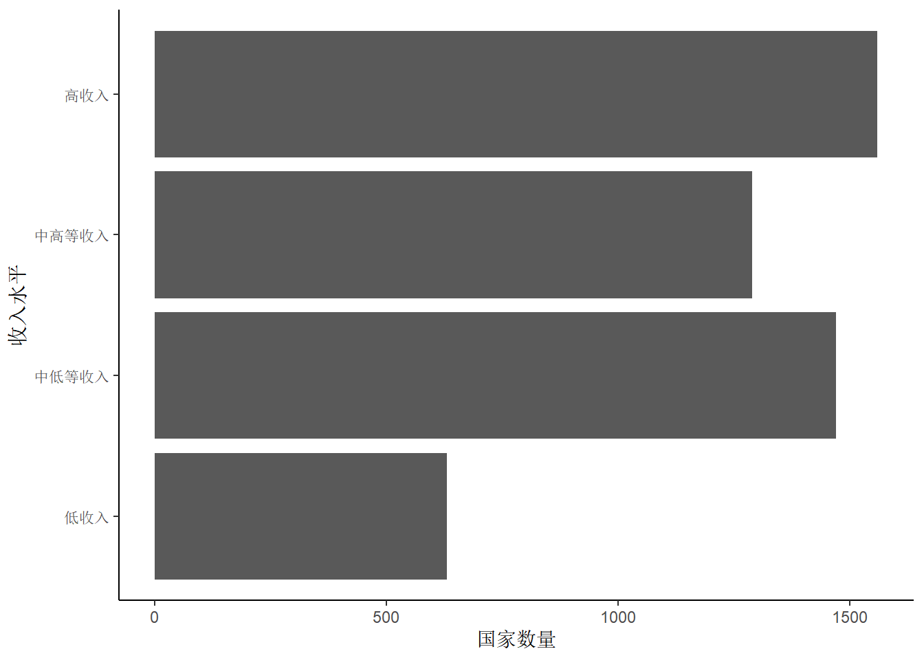
1 坐标系统
不同坐标系下的柱状图、条形图、饼图。
Note
值得注意的是,ggplot2中没有直接绘制饼图的函数(Hadley认为饼图并不能很好的展示数据),只能通过极坐标转换。
library(scales)
gapminder_2007 <- gapminder %>%
filter(year == 2007)
ggplot(gapminder, aes(x = income_level)) +
geom_bar(stat = "count") +
theme_classic() +
labs(x = "收入水平", y = "国家数量")
ggplot(gapminder, aes(x = income_level)) +
geom_bar(stat = "count") +
coord_flip() + # 坐标轴翻转
theme_classic() +
labs(x = "收入水平", y = "国家数量")
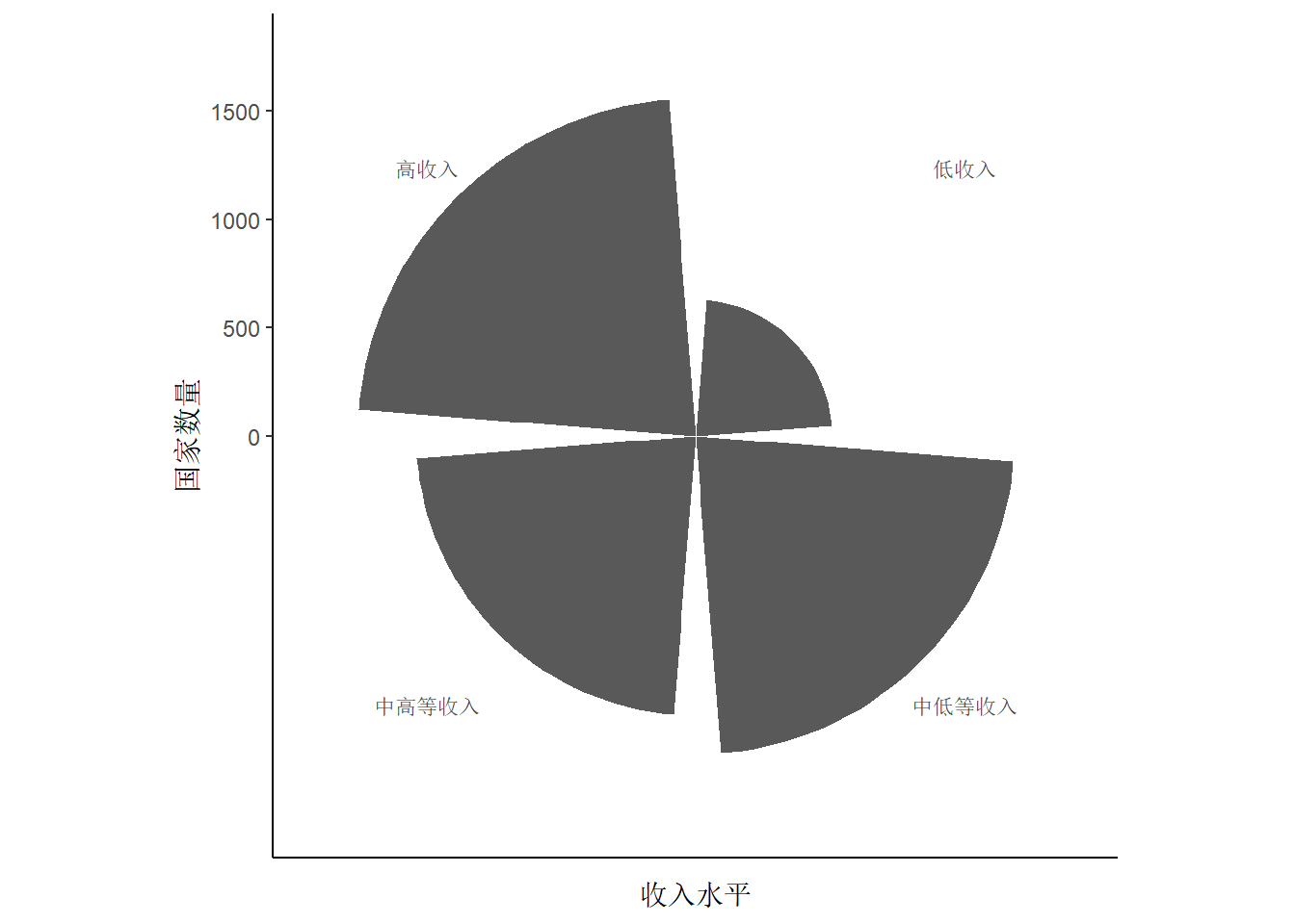
ggplot(gapminder, aes(x = income_level)) +
geom_bar(stat = "count") +
coord_polar(theta = "x") + # 极坐标转化:x轴转化,其中参数theta="x"可省略
theme_classic() +
labs(x = "收入水平", y = "国家数量")
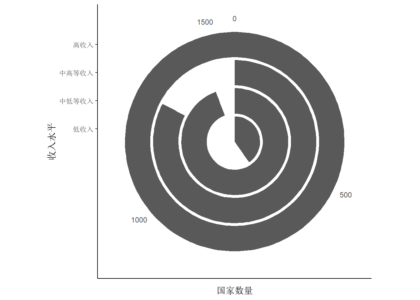
ggplot(gapminder, aes(x = income_level)) +
geom_bar(stat = "count") +
coord_polar(theta = "y") + # 极坐标转化:y轴转化
theme_classic() +
labs(x = "收入水平", y = "国家数量")
以上图形中均可以加入分组情况,如希望按照地区分组,只需在参数aes()中加入fill=region即可。
2 插入公式
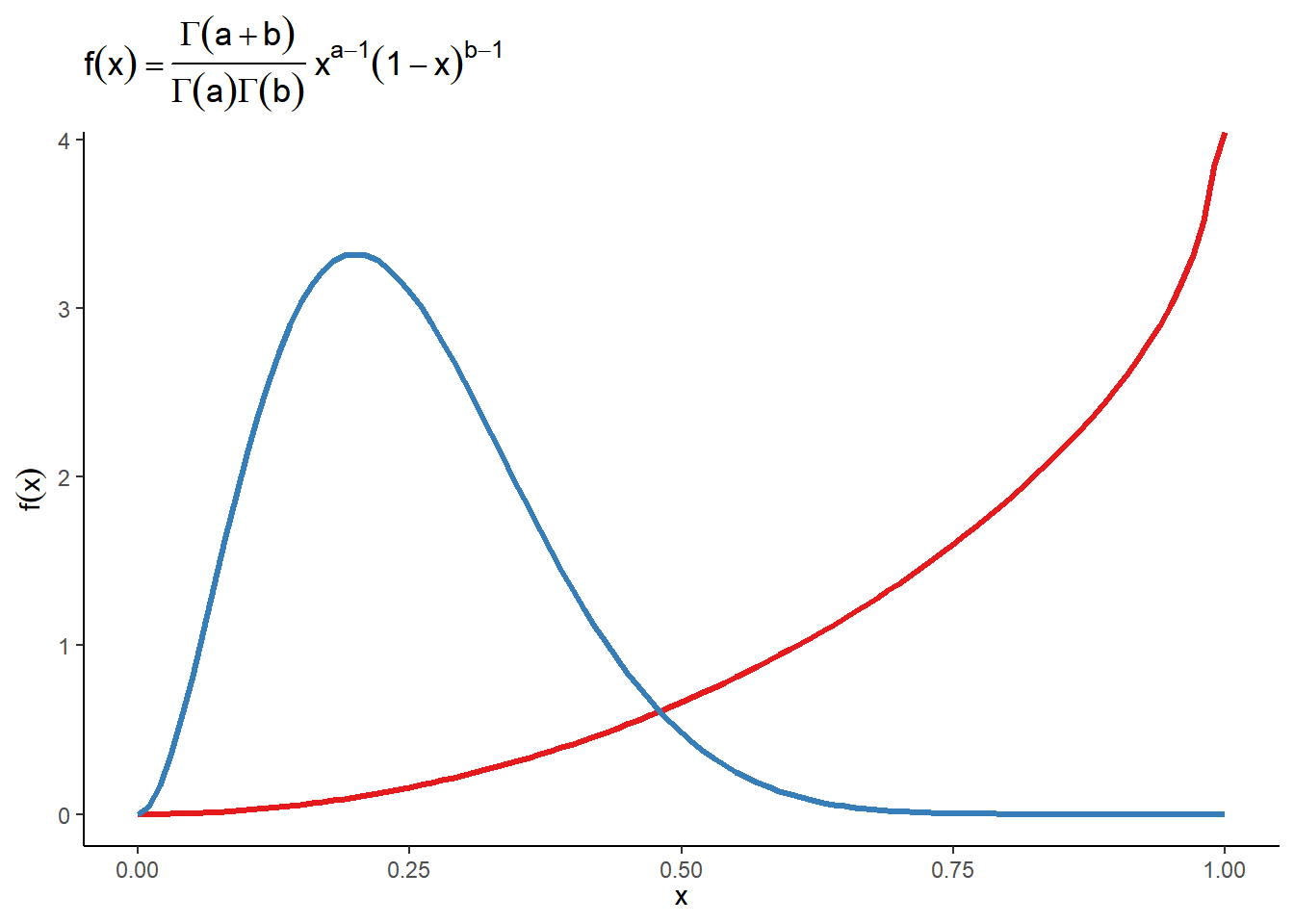
有时,我们需要在图片中插入公式使得图片的展示效果达到最佳。相比ggplot2中自带的插入公式的方法,我更习惯latex2exp输入的公式的方式。
例如,我们如何在ggplot2图形中插入如下公式(形状参数分别为a和b的贝塔分布的概率密度函数):
\[ f(x;a,b)=\frac{\Gamma(a+b)}{\Gamma(a)\Gamma(b)}x^{a-1}(1-x)^{b-1}, \quad a>0,b>0,0\leq x \leq 1 \]
library(latex2exp)

ggplot() +
  geom_function(
    fun = dbeta, args = list(shape1 = 3, shape2 = 0.9),
    colour = "#E41A1C", linewidth = 1.2,
  ) +
  geom_function(
    fun = dbeta, args = list(shape1 = 3, shape2 = 9),
    colour = "#377EB8", linewidth = 1.2
  ) +
  theme_classic() +
  labs(
    x = TeX(r'($x$)'), y = TeX(r'($f(x)$)'),
    title = TeX(r'($f(x)=\frac{\Gamma(a+b)}{\Gamma(a)\Gamma(b)}x^{a-1}(1-x)^{b-1}$)')
  )
3 散点图
观察变量之间的关系,可以使用geom_point()函数。
titanic <- titanic[complete.cases(titanic), ] # 删除缺失值,这段代码的作用是删除 "titanic" 数据框中包含缺失值的所有行,结果仍然保存在 "titanic" 变量中。

# 基础散点图
fig(12, 8)
ggplot(titanic, aes(x = Age, y = Fare)) +
  geom_point(aes(color = Sex)) + # 按照性别分组
  theme_classic() +
  theme(plot.title = element_text(size = 22)) +
  labs(x = "年龄", y = "票价")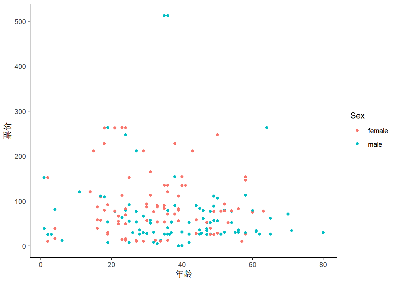
# 多个变量间的散点图
ggplot(university, aes(x = quality_of_education, y = score)) +
  geom_point(aes(color = country, size = citations)) +
  labs(
    x = "Quality Of Education",
    y = "Score",
    title = "Quality of Education Vs Score against Country & Citations"
  ) +
  theme_linedraw() +
  theme(
    plot.title = element_text(size = 22), axis.text.x = element_text(size = 15),
    axis.text.y = element_text(size = 15), axis.title = element_text(size = 18)
  )
# 抖动散点图
costly_price_with_less_area <- house |>
  filter(SalePrice > 600000 & LotArea < 25000)

ggplot(house, aes(x = LotArea, y = SalePrice)) +
  geom_jitter(aes(color = LotShape), alpha = 0.5, width = 0.5, size = 2) +
  # 在 LotArea 和 SalePrice 的散点图上,
  # 用一个环形区域突出显示出costly_price_with_less_area显示范围内的房屋数据
  geom_encircle(aes(x = LotArea, y = SalePrice, color = LotShape),
    data = costly_price_with_less_area, size = 1.5, expand = 0.08
  ) +
  theme_bw() +
  theme(plot.title = element_text(size = 22)) +
  labs(x = "LotArea", y = "SalePrice")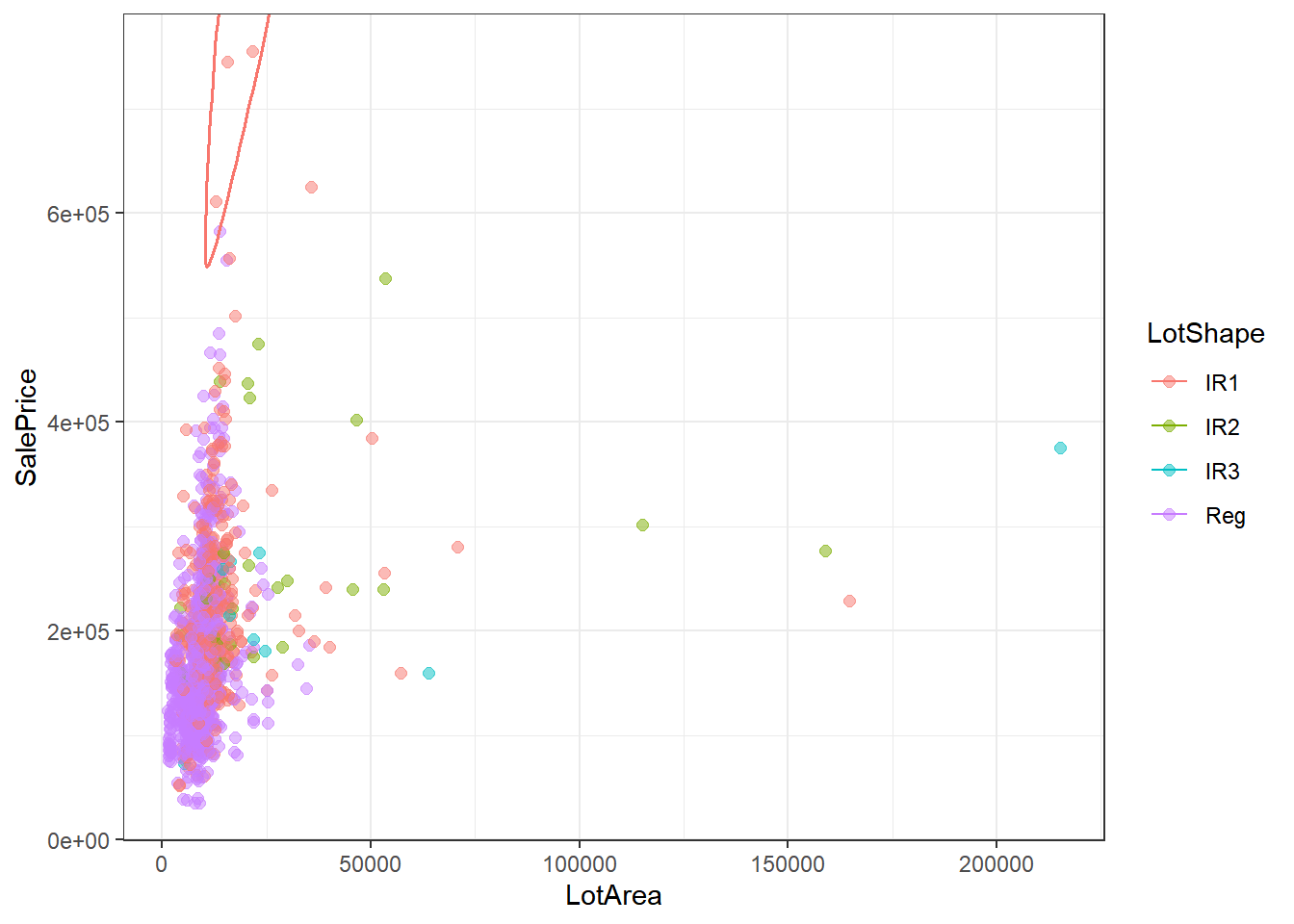
4 气泡图
# 数据预处理
set.seed(1234)
age1 <- health |>
  separate(Age, into = c("X1", "X2"), sep = "-") |>
  select(X1, X2)

stay1 <- health |>
  separate(Stay, into = c("X3", "X4"), sep = "-") |>
  select(X3, X4)

health_df <- cbind(age1, stay1, health$Admission_Deposit, health$`Severity of Illness`) |>
  rename(
    Age_Start = X1, Age_End = X2, Stay_Start = X3, Stay_End = X4,
    Deposit = "health$Admission_Deposit",
    Severity = "health$`Severity of Illness`"
  ) |>
  mutate(
    Age_Start = as.numeric(Age_Start), Age_End = as.numeric(Age_End),
    Stay_Start = as.numeric(Stay_Start), Stay_End = as.numeric(Stay_End),
    Deposit = as.numeric(Deposit)
  )

health_df <- health_df[complete.cases(health_df), ] # 删除缺失值

health_df <- health_df |>
  rowwise() |> # 按行操作
  mutate(
    age = sample(seq(Age_Start, Age_End), 1), # 从Age_Start到Age_End中随机抽取一个数
    stay = sample(seq(Stay_Start, Stay_End), 1) # 从Stay_Start到Stay_End中随机抽取一个数
  ) |>
  ungroup() # 取消按行操作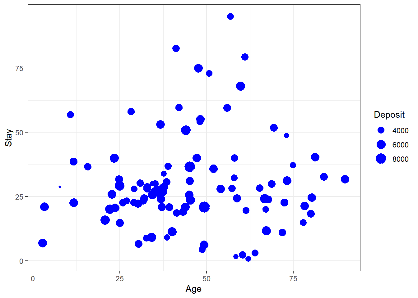
5 柱形图
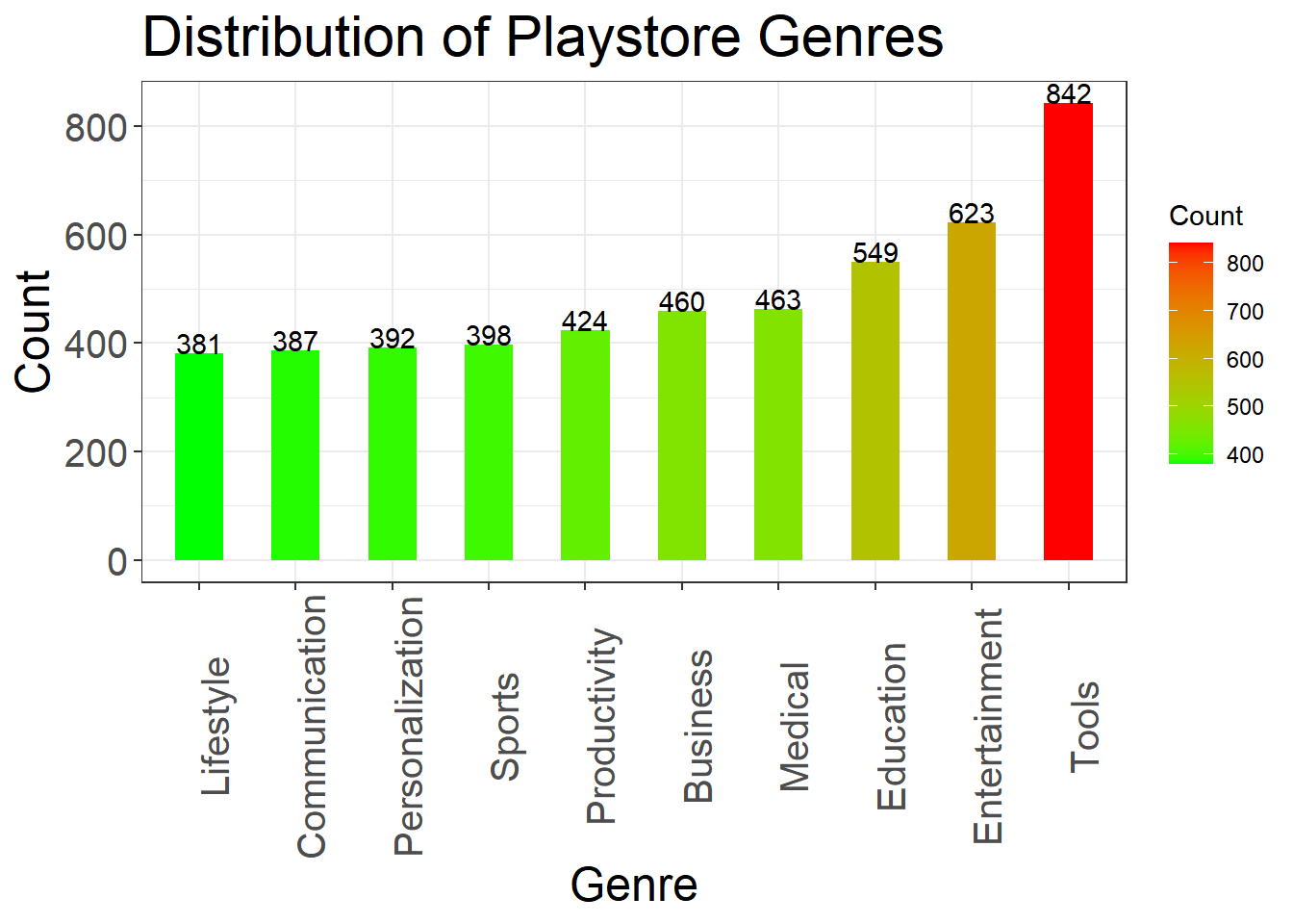
# 基础柱形图-图形条渐变和文本
genre_data <- as.data.frame(table(playstore$Genres))
genre_data <- genre_data[order(-genre_data$Freq), ] |>
  top_n(10)
colnames(genre_data) <- c("Genre", "Count")

ggplot(genre_data, aes(reorder(Genre, Count), Count, fill = Count)) + # 按照Count降序排列
  geom_bar(stat = "identity", width = 0.5) +
  # 图形条文本
  geom_text(aes(label = Count), vjust = 0) +
  # 图形条颜色渐变
  scale_fill_gradient(low = "green", high = "red") +
  labs(
    x = "Genre",
    y = "Count",
    title = "Distribution of Playstore Genres "
  ) +
  theme_bw() +
  theme(
    plot.title = element_text(size = 22),
    axis.text.x = element_text(size = 15, angle = 90),
    axis.text.y = element_text(size = 15),
    axis.title = element_text(size = 18)
  )
# 堆叠柱形图
ind_us_shows <- netflix |>
  filter((country == "United States" | country == "India") &
    release_year > 2015)
ggplot(ind_us_shows, aes(release_year, fill = country)) +
  geom_bar(stat = "count", position = "stack") + # stack表示堆叠,dodge表示并列
  labs(
    x = "年份",
    y = "数量",
    title = "网飞在印度和美国的数量分布"
  ) +
  theme_bw() +
  theme(
    plot.title = element_text(size = 22),
    axis.text.x = element_text(size = 15),
    axis.text.y = element_text(size = 15),
    axis.title = element_text(size = 18)
  )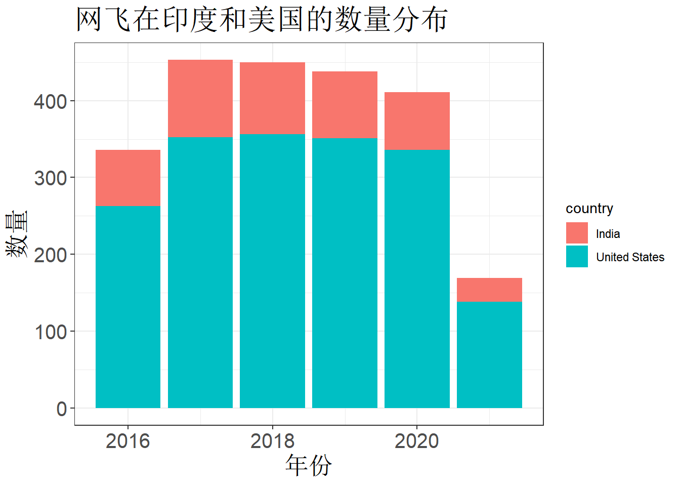
ggplot2中没有饼图,可以使用geom_bar()和coord_polar(),通过转换坐标系来绘制饼图。
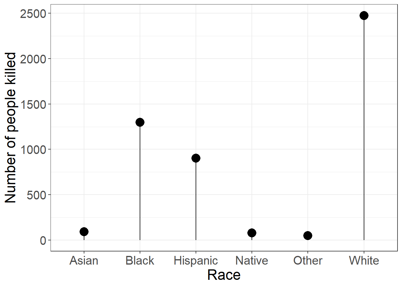
6 等级图 (Rank Chart)
6.1 棒棒糖图
as.data.frame(table(police$race)) |>
  rename(race = Var1, count = Freq) |>
  # 棒棒糖图为点图和线图的结合
  ggplot(aes(race, count)) +
  geom_point(size = 5) +
  geom_segment(aes(x = race, xend = race, y = 0, yend = count)) +
  labs(
    x = "Race",
    y = "Number of people killed"
  ) +
  theme_bw() +
  theme(
    axis.text.x = element_text(size = 15),
    axis.text.y = element_text(size = 15),
    axis.title = element_text(size = 18)
  )
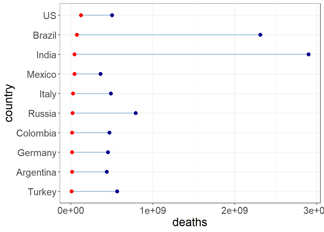
6.2 哑铃图
covid |>
  group_by(`Country/Region`) |>
  summarise(
    deaths = sum(Deaths),
    recovered = sum(Recovered)
  ) |>
  arrange(desc(recovered)) |>
  slice_head(n = 10) |>
  rename(country = `Country/Region`) |>
  mutate(
    country = fct_reorder(country, deaths)
  ) |>
  ggplot(aes(deaths, xend = recovered, y = country, group = country)) +
  geom_dumbbell(
    size = 0.75, color = "#a3c4dc", size_x = 2.5, size_xend = 2.5,
    colour_x = "red", colour_xend = "darkblue"
  ) +
  theme_bw() +
  theme(
    axis.text.x = element_text(size = 15),
    axis.text.y = element_text(size = 15),
    axis.title = element_text(size = 18)
  )